Advances in dual energy computed tomography approach for proton stopping power ratio computation in radiotherapy

Abstract

To address the sensitive and uncertain limitations of single-energy computed tomography (CT) calibration methods in computing proton stopping power ratio during treatment planning, different methods have been proposed using a dual energy CT approach. This paper reviews the most recent dual-energy CT approaches for computing proton stopping power ratio. These include image domain and projection domain methods. The advantages and uncertainties of these methods are analyzed based on existing studies. This paper highlights recent advances in dual energy CT, discussing their implementation, advantages, limitations, and potential for clinical adoption.

Key Words: Dual energy computed tomography; Stopping power ratio; Machine learning; Mathematical model; Image domain; Projection domain; Radiotherapy; Alternating minimization algorithm; Electron density; Mean excitation energy

Core Tip: This literature presents different methods of calculating proton stopping power ratio using dual energy computed tomography data. It outlines the implementation of different algorithms, review different research works and propose further research works that need to be carried out to facilitate the clinical implementation of dual energy computed tomography approach to improve ion therapy.

INTRODUCTION

Proton therapy and other heavy ion therapies are gaining popularity in tumor treatment. The treatment planning parameters, like proton stopping power ratio (SPR), are mostly calculated from computed tomography (CT) data. The single-energy CT (SECT) method proposed by Schneider et al[1] is the most commonly used approach for computing proton SPR in clinical settings; however, it is prone to significant uncertainties. The two types of uncertainties that exist in real world are: Internal uncertainties within the recommended values, which can be up to a few percent and individual patient-to-patient variation[2]. International Commission on Radiation Units and Measurements Report No. 44 clearly states that ‘the elemental compositions of most body tissues are known to vary considerably between individuals of the same age’ and the composition of a given individual may vary from one body site to another[3]. In order to mitigate these uncertainties, the dual-energy CT (DECT) approach was proposed with the idea of using two energy data to compute two parameters which are relative electron density (ρ_e) and mean excitation energy (I) that are used to compute SPR in Bethe-Block equation[2]. The concept of using DECT to calculate both relative electron density and effective atomic number (Z) was first introduced by Rutherford et al[4], at around the time the CT scanner was invented. Using DECT to estimate photon cross sections at low energy in the range of 20-1000 keV was also proposed by Williamson et al[5].

To realize the full potential of proton therapy, the range of the proton beam, which is defined as the depth of the Bragg peak, needs to be accurately determined[6]. Some factors like random noise as well as residual systematic errors in the separately reconstructed CT images like HU non-uniformity and dependence on patient size due to residual beam-hardening and scatter artifacts, may cause accuracy of SPR estimates derived from image-domain analyses to deteriorate in the clinical setting[7-9]. This leads to projection-domain approach which uses CT projection data instead of CT-image.

The idea of using DECT to resolve the non-bijective relation found in HU-ρ_e and HU-SPR relations by computing Z has been questioned. One being that the value of Z for a given material is energy- and definition-dependent[10-13] and thereby questions its consideration as physical property leading to accurate and robust tissue characterization. This leads to atomic composition approach through segmentation like the one presented by Landry et al[14] and Lalonde and Bouchard[15]. Lalonde and Bouchard[15] applied principal component analysis on tissue elemental composition in order to calculate the photon mass energy absorption coefficient and SPR for Monte Carlo dose calculation using dual and multi-energy on a set of 71 human tissues from two publications by Woodard and White[16] and White et al[17]. Including this approach, most tissue characterization methods proposed in literature can be classified into three categories: Segmentation, parameterization and decomposition category for the case of image domain.

In this presentation, we focused mainly on parametrization and decomposition category because they are presented in the five papers we are reviewing in details. These methods are presented in two approaches which are image and projection domain approach. The implementation of the methods is discussed and reviewed in line with the literature presented by Yang et al[2], Zhang et al[18], Lee et al[19] and Chika[20,21] as well as others. These literatures were chosen based on their in-depth study, widely used results or recent novel approaches applied in the study like machine learning and deep learning.

PROTON SPR ESTIMATION MODEL

In theoretical simulation, reference SPR (or sometimes called true SPR) is mostly estimated using Bethe equation or Bethe-Block equation. The equations are stated below for the range of energy used in proton therapy.

Model 1 (Bethe equation)

The proton stopping power can be approximated using the Bethe equation[22].

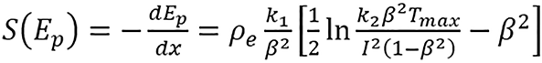(1).

For a given energy E_p, where k₁ and k₂ are products of physical constants; β = v_p/c is the proton speed relative to light; T_max is the maximum energy transferred from the proton to a single electron; and ρ_e and I are the electron density and mean excitation energy of the medium, respectively. SPR is computed by dividing stopping power of the medium with that of water, i.e., SPR = [S(E_p)]/[S_w(E_p)], where S(E_p) is the stopping power of the medium and S_w(E_p) is the stopping power of water.

Model 2 (Bethe-Block equation)

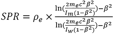
The Bethe-Block equation[23] can be used to compute proton SPR, this can be approximated by:

(2),

where m_e is the electron mass, cβ is the velocity of the proton beam, I_m and I_w are the mean excitation energies of the mixture and water, respectively.

DUAL ENERGY METHODS OF COMPUTING PROTON SPR

Methods presented in at least one of the five papers that will be discussed in more details are presented in this section. It will be divided into image domain and projection domain methods.

Image domain methods

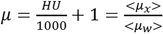
The image domain methods presented mainly use two forms of modified CT numbers as input data[7,24-26]. The modified CT numbers are as follows:

(3),

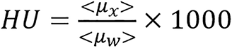(4),

where μ_w represents linear attenuation of water and μ_x represents linear attenuation of the medium/tissue. Sometimes, this can be generally represented by

(5),

where A and B are determined from calibration.

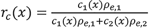
Basis vector model/method: This model uses two dissimilar basis to represent the energy-dependent photon cross sections of biological media. This can be written in terms of linear attenuation for dual energy as c₁(x)μ_1,L(E) + c₂(x)μ_2,L(E) = μ_L(x,E), c₁(x)μ_1,H(E) + c₂(x)μ_2,H(E) = μ_H(x,E). The component weights, c_i(x) for an unknown material at image pixel x are then determined from

(6),

where μ_i,L/H are the modified HUs of the basis materials obtained from calibration images at low and high energies.

(7),

(8),

and the I can be estimated using basis material weight[6,24] with either of the following:

(9a)

or

(9b)

where

,

,

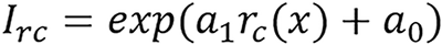
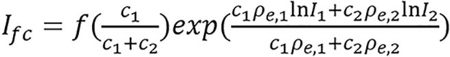
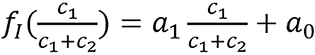
a₀ and a₁ are constants to be determined through calibration from the given mean excitation energy and

is referred to as an empirical correction function of ρ_eI_fc = c₁ρ_e,1lnI₁+ c₂ρ_e,2lnI₂. ρ_e,i and I_i are electron densities and mean excitation densities of the two basis materials, respectively, i = 1, 2. Basis material selection is presented by Williamson et al[5] and Han et al[24].

Hunemohr’s and Saito model: Dual energy model for computing relative electron density and effective atomic number was presented by Hünemohr et al[25]. Saito[7] developed similar formula for computing ρ_e, hence it is sometimes referred to as Hunemohr’s and Saito model (H-S model also called H-S method).

(10),

(11),

where μ_L and μ_H are the modified HU. This modified HU is proportional to the spectrally averaged attenuation coefficient. The constants, a and b depend on the specific dual-energy scanning protocol.

(12),

where ω_k, Z_k, and A_k are the mass fraction, atomic number and atomic weight of the k^th element in the material, respectively; ρ_e,w and Z_eff,w are electron density and effective atomic number of water respectively.

Bourque’s model/method: Spectrally averaged elemental electronic cross-sections are fit to a polynomial function as proposed in Bourque et al[13],

,

of their atomic numbers Z. The spectrum-dependent effective atomic number for an arbitrary mixture is defined as

.

The parametric ρ_e - Z_eff model is given by:

(13),

(14),

where c_k and b_m,L/H are scanner-specific model parameters. The orders of polynomial fitting used in their study are K = M = 6. In this model, first step is to calculate Z_effvia equation (13). Using equation (14), two different estimations of ρ_e are computed from images of low and high energies, respectively, and the final estimated value of ρ_e is obtained by taking their average.

Torikoshi-Bazalova method: The monochromatic form of this method was presented by Torikoshi et al[26] and extended to polychromatic by Bazalova et al[27], hence, it is labeled the Torikoshi-Bazalova method. This was used to compute proton SPR in Yang et al[2]. For monochromatic phonton beam of energy below 1.02 MeV, an arbitary element total linear attenuation coefficient can be approximated by Torikoshi et al[26].

μ = ρ_e [Z⁴F(E,Z) + G(E,Z)] (15), where ρ_e, Z and E are the electron density, atomic number and beam energy, respectively. ρ_eZ⁴F(E,Z) and ρ_eG(E,Z) represent the photoelectric attenuation and the combining term of Compton scatter and coherent scatter attenuation respectively. The interpolation of the element’s photoelectric and scattering attenuation coefficients can be used to determine the values of F(E,Z) and G(E,Z) for element Z at arbitrary energy E.

The linear attenuation coefficient of an unknown material for a polychromatic beam can be approximated by:

(16),

where k denotes different X-ray spectra and w_k,i is the weighting function of the k^th energy spectrum. The quantities in bracket are averaged over the k^th spectrum. Combine equations (15) and (16) to obtain,

(17),

the following notations were made, where the subscript w represents the value for water. Let

,

,

,

.

Then, equation (17) becomes

(18),

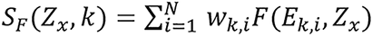
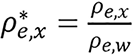
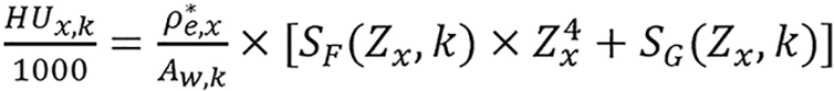
ρ^*_e,x and Z_x are the two unknowns in the equation. By assuming that S_F(Z_x,k) and S_G(Z_x,k) do not depend on the Z_x strongly,

can be iteratively determined by solving

(19),

where

,

with the known value of Z_x, ρ^*_e,x can be determined using the data of either energy spectrum by

(20).

The accuracy of the algorithm depends on the CT numbers and the beam energy spectra but not on physical CT scanner setup. Given two CT measurements of the same material and the corresponding beam energy spectra, ρ_e and Z_eff can be computed using the algorithm.

Taasti method: Taasti et al[28] presented empirical parametrization model using dual energy as stated below.

(21).

(22).

The constants a_k are determined separately for soft and bone tissues.

Chika CE method: This method was developed by Chika[20] for estimating different radiological parameters using multi-energy, this method involves the use of mathematical model and algorithm. The restricted version of the method for computing SPR using dual energy is discussed in this paper. The algorithm will be discussed while reviewing the paper in the next section. The model is as stated below:

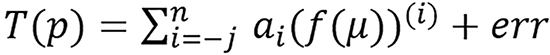
Given a radiological parameter p related to the attenuation coefficient μ, there exist transformations/maps T(p) and f(μ) such that

(23),

n ≥ 0, j ≥ 0 and p = T^-1(T(p)),a_i ∈ R, where μ = (μ₁, μ₂, μ₃, …, μ_m) for m-energies (m ≥ 1) with at least one low energy (that is ≤ 90 kVp) and err is an acceptable error. The paper used three f(μ) for dual energy which are f_L(μ) = μ_L, f_r(μ) = μ_L/μ_H, f_m(μ) = μ_L*μ_H. Symbol definition: T_p,j,n means T for parameter p, low index -j and top index n. That is, in terms of SPR as follows:

Projection domain methods

Two projection domain approaches are presented.

Sinogram-domain decomposition method: This approach aims to extract two line integral components which are invariant to spectral variations before reconstructing the image. Filtered back projection (FBP) or other methods are used to reconstruct the two corresponding component images after the decomposition.

Let ψ_j(y,E), j∈{L,H} such that ∑_E ψ_j(y,E) = 1 be the detector response-weighted spectrum of the low- and high- energy scans for photon energy E and source-detector pair y, let I_0,j(y) be the corresponding detector response in the absence of a scan subject expressed in noise-equivalent quanta. The expected transmission sinogram for an attenuating object can be modeled as follow:

(24),

where μ_(x,E) is the photon linear attenuation coefficient of energy E at image pixel x and h(y,x) is the point-spread function of the scanner system which represents the effective length of the intersection between the path y and image pixel x.

The energy uncompensated measurement d_j(y) is assumed to equal the expected mean Q_j(y) and based on the basis vector model/method (BVM) the two line integrals corresponding to the two bases are defined as: L_i(y) = ∑_x h(y,x)c_i(x) (25), which implies that

(26),

L_j(y) can be solved from equation(26) for each source-detector pair y independently using Newton’s method or it can be solved using line integral alternating minimization algorithm as presented in the Supplementary material.

Dual energy joint statistical image reconstruction method: Joint statistical image reconstruction (JSIR) method is combined with BVM to form JSIR-BVM method[18,29,30]. JSIR-BVM method for SPR estimation presented by Zhang et al[18] is based on the dual-energy alternative minimization (DEAM) algorithm[29,30] which reconstructs the two images BVM component weights directly and simultaneously from the two energy-uncompensated sinograms d_L(y) and d_H(y). In DEAM algorithm, the reconstruction process is based on the statistical model of CT data which is formulated as a penalized maximum likelihood estimation problem. The measured transmission data d_j(y) are assumed to be independently Poison distributed with the expected mean parametrized by BVM component weights as:

(27).

The two BVM component images are found by minimizing the following objective function:

(28).

Maximization of the log-likelihood of c_i is equivalent to minimization of the I-divergence[31] between the measured transmission data d_j and the estimated mean values Q_j over c_i[6,32],

(29).

The first term in the objective function [equation (28)] is the data-fitting term. The second term is a regularization term that enforce smooth images by penalizing the difference between neighboring pixels. R(c_i) is the spatial penalty function formulated as

(30),

where

(31).

The adjacent neighborhood of pixel x is denoted by ℵ(x) and w_x,k represents an inverse distance weight for each pixel pair. Ф_(t) is the Huber-type potential function which has a quadratic region for |t| < 1/δ and a linear region for |t| > 1/δ, which is able to preserve edges while suppressing noise[33]. The parameter λ in equation (28) controls the trade-off between data fitting and image smoothness. A large λ produces images with smaller noise level but lower resolution. The details of DEAM algorithm derivation used in solving the problem can be found in O’Sullivan et al[30] and it’s presented in the Supplementary material. Some acceleration techniques such as ordered subset[34] and heuristic step size can be applied.

Stochiometric method

The most popularly used method for treatment planing is the SECT calibration method. Based on this, it’s normally used for comparison. Therefore it’s presented here. Single energy calibration method uses single energy attenuation to estimate SPR through linear piece wise function, that is,

(32).

DISCUSSION/REVIEW

DECT and SECT variance analysis

Yang et al[2] presented theoretical variance analysis of single and dual energy CT methods for calculating proton SPRs of biological tissues. Considering that variation of human tissue composition depending on health condition, genetics, gender, age and other factors is well known, they considered the effect of variation in tissue composition for SPR accuracy. The study was carried out using Torikoshi-Bazalova method.

The CT number defined in equation (4) was used in their study. The linear attenuation coefficient <μ_x> of a single element was calculated by:

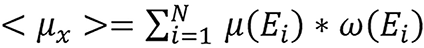(33),

where μ(E_i) is linear attenuation coefficient and ω(E_i) is the weight in the beam spectrum for energy E_i.

It was found that spectrum change has a large impact on bone tissues and the difference is in hundreds of HUs. The work showed that the bone tissues CT numbers are very susceptible to spectrum change, particularly at the low energy range; it also shows that it’s necessary to have additional water filtration inorder to simulate the spectrum change along the beam path in patient geometry. The spectra of 100 kVp and 140 kVp were used to calculate the CT numbers for DECT method, and 120 kVp spectrum were used to compute those for stoichiometric calibration method.

The work (figure 2 in their paper) shows that the relative errors in calculated Z_eff of most tissues are between -1% and 1%, i.e., (-1, 1)%. The only outlier for this range of error is thyroid which contains 0.1% iodine. The relative errors in calculated ρ_e of all tissues are between -0.35% and 0.35%, i.e., (-0.35, 0.35)%. Although they reported this as less than ± 1% and less than ± 0.35%, respectively, which were not correct representation of the result since less than -1% implies it takes values from -100% to -1% similarly less than -0.35% implies it takes values from -100% to -0.35%.

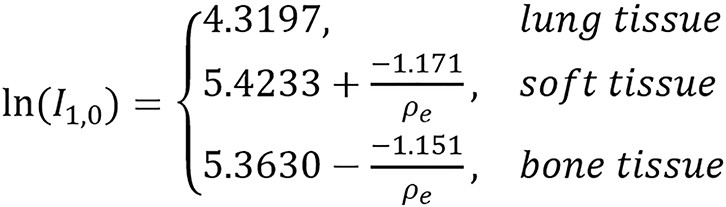
Proton SPR was computed using equation (2) and the proton beam energy used in the study was 175 MeV. The relationship between effective atomic number (Z_eff) and mean excitation energy (I) was introduced in the paper and can be represented as follows:

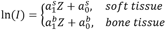(34).

Different fitting can be done for lung tissue since the tissues are normally grouped into lung tissue, soft tissue and bone tissue. lnI was calculated using the Bragg additivity rule by:

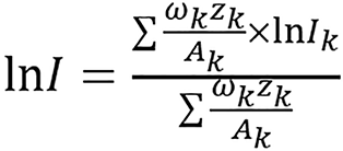(35),

where ω_k, Z_k, A_k, and I_k are the mass weight, atomic number, atomic mass and mean excitation energy of the ith element, respectively[23,35]. The Z_eff of a composite material was calculated using equation (12) and was computed from CT numbers using the DECT algorithm for standard human biological tissues which n was found to be 3.3. In each tissue group (soft and bony tissue groups), lnI has a good linear relationship with Z_eff except thyroid tissue which contains 0.1% iodine and was omitted from the linear fitting.

Various levels of variations to density and elemental composition of standard human biological tissues were introduced to study the sensitivity of the method and stochiometric calibration method. For variation in density, either increase or decrease of the original value by a certain percentage (α%). For elemental composition, choose one element from each of the three elements with highest proportion (which are oxygen, carbon and hydrogen for soft tissue, oxygen, carbon and calcium for bone tissue) and add or subtract its percentage by a fixed percentage (α%). To study partial volume effect, two human biological tissues were mixed in equal volumes. The comparison was done using the SPRs estimated from both methods to their theoretical values. Often in CT images, a partial volume artifact occurs as a result of voxels containing more than one type of tissue, for instance soft tissue near a bony edge. DECT methods gives much lower errors in SPR estimation compared to the stoichiometric calibration method: The maximum error and the root mean square error (RMSE) are reduced from 3.24% and 0.89% to 1.00% and 0.26%, respectively. The study shows that the accuracy of the DECT method was less susceptible to the component variation when compared to the stoichiometric calibration method. The percentage change in carbon and oxygen was found to have almost no impact on the accuracy of estimated SPR on either the DECT method or the stoichiometric calibration method. For the partial volume effect, the accuracy of the SPR estimated using the stoichiometric calibration method was substantially decreased, with maximum error increasing from 3.24% to 33% and the RMSE from 0.89% to 4.35% for SECT, but for DECT method, the mixing has very limited impact on the accuracy of SPR estimated.

The study showed that there will be a deterioration on the accuracy of the DECT method and the stoichiometric calibration method when density or major elemental components deviate from those of the standard human tissues[2]. They claimed that they were not able to find any comprehensive study to estimate the range of density and elemental component variations in human tissues so they couldn’t survey the possible range of variations for these deviations in reality, though, they presented some literature review on some publications that touched the topic. They also mentioned that the data available as at the time of the work do not include spatial variations within the same human tissue. Linear correlation between the density and calcium for bone tissues was described. The study makes use of theoretical CT number which does not include so many practical uncertainties. Also, more comprehensive study on possible variations on density and human tissue composition is needed for more practical study of the uncertainties. Carrying out more studies on projection domain approach may be able to improve this uncertainty due to variation in tissue composition.

Image and projection domain comparative analysis

In Zhang et al[18] paper, impact of JSIR method was studied for reconstruction of proton power images and comparison of some image and projection domain methods was presented. Equation (1) was used to compute reference SPR at Ep = 200 MeV. 34 International Commission on Radiation Units and Measurements reference human tissues[3,17] was used for calibration. Photon mass attenuation coefficients were gotten from National Institute of Standards and Technology XCOM data[36] and mixture rule was applied to it to calculate linear attenuation. Theoretical CT numbers were calculated by taking the average over the known X-ray energy fluence spectrum ψ(E) as <μ> = ∫_E ψ(E)μ(E)dE and using equation (3). Birch-Marshall model[37] was used to compute low and high energy spectrum for 90 kVp and 140 kVp tube potentials with 12 mm Al filtration. The image methods presented were BVM, H-S method and Bourque’s method while the projection domain methods presented were JSIR and sinogram-decomposition domain method.

For the BVM, polystrene and CaCl₂ solution (23% concentration by mass) were used. FBP algorithm was used for reconstruction after applying water based beam hardening correction[38,39] to each synthetic polychromatic sinogram. The BVM components weights were estimated from equation (6) by least-square-fitting weighted by the source spectrum and I_fc was used.

For Hunemorh’s model, 3.2 was found to be the optimal value of n for CT spectra assumed in their simulation. This optimal value was found by fitting the attenuation coefficients of elements for Z = 2-20. In implementation of Bourque’s model, K = M = 6 was used just as in original study. They made use of the numerical/emprical relationship between I-value and Z_eff which was first introduced by Yang et al[2]. In Sinogram-domain decomposition approach, Li(y) were solved from equation (26) for each source-detector pair y independently using Newton’s method and the BVM components weights, c_i(x), were obtained from L_i(y) using the FBP algorithm. ρ_e and I-value can be estimated using equations (7) and (8). They extended the two calibration based ρ_e - Z_eff models into the sinogram-domain decomposition approach[40] using computing two monochromatic HU images at the effective energies of low and high energy scans for both calibration and test phantoms, the effective energy for 90 kVp spectra is 55 keV and the effective energy for 140 kVp spectra is 69 keV; this helps to comprehensively compare with the image domain on the study. In dual energy JSIR approach, DEAM algorithm was used with 600 iterations for δ = 100 and λ= 6.

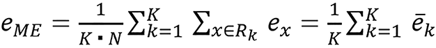
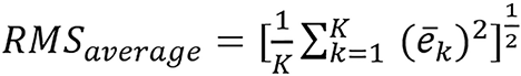
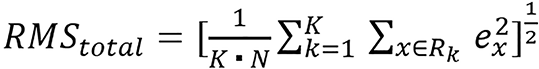
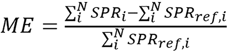
They studied six different combinations and JSIR-BVM methods. They combined the three image methods they studied with FBP constructed images and sinogram-domain decomposition approach to form the other six methods. For accuracy analysis, the mean error (e_ME), the RMSE of tissue-specific average errors (i.e., RMS_average), and RMSE over all region of interest pixels (RMS_total) are as follows:

(36),

(37),

(38),

where R_k is the region of interest of the k^th tissue, N is the number of pixels in each region of interest, e_x is the relative SPR estimation error at pixel x, and

is the average estimation error for the k^th tissue. ME indicates the overall bias of the predicted SPR, RMS_average error measures the systematic estimation error variation for different tissues, and RMS_total error reflects the pixel-to-pixel variation in the SPR image.

The JSIR method was shown to achieve more accurate reconstructions and more effective in suppressing artifacts. CT image noise and residual beam-hardening artifacts are propagated into the converted SPR images and high image noise compromised the quality of the SPR images derived from the FBP based image and sinogram-domain decomposition methods. Their study considered different impacts, such as impact of reconstructed image intensity uncertainty on SPR estimation (which includes noise levels) and the impact of test object geometry on SPR estimation. The study found that the most robust in the presence of noise among the six image and sinogram-domain decomposition methods considered is the BVM based sinogram-domain decomposition method. Also, the RMS-average errors of the JSIR-BVM method from the same source intensity level are less than 1/6 of those of all the other six methods.This shows that in homogeneous region, JSIR-BVM method has much smaller pixel-to-pixel SPR variations compared to the other two approaches. Hence, under different noise levels the JSIR-BVM method achieves high mean estimation accuracy in addition to dramatically reducing the statistical uncertainty of SPR estimates.

They observed that CT numbers of the larger phantom are generally lower than those on the smaller phantom for the two separately reconstructed images. CT numbers increase with the distance to the phantom center on the same phantom. This is in line with known fact which is that the equivalent spectrum passing through the center of a large phantom is harder than that passing through the border of a small phantom. Their result suggested that the HU differences caused by the residual beam hardening effects in the single energy reconstructed images are the dominant contribution to the systematic variation of SPR estimates. Since image domain decomposition methods rely on two separately reconstructed CT images, residual beam hardening effects introduce image intensity uncertainties as well as other image artifacts, leading to systematic SPR estimation error much larger than the intrinsic modeling error, thereby limiting the benefit of DECT in mitigating proton range uncertainty. Noticeable uncertainties in the SPR predictions of the test objects can be introduced by test object variability and CT number variations of the calibraton phantoms. Rearrangement of the Gammex inserts in the calibration phantom according to the study alters soft and bone tissue SPR estimates by some percentages that are up to 0.4% and 0.8%, respectively. It has also been shown in the study by Li et al[9] that the selection of calibration materials may affect the estimation results. The presented result in the work demonstrates that the JSIR-BVM method supports accurate SPR mapping for various object geometries and outperforms other investigated methods in terms of robustness to noise. Sinogram-based and joint reconstruction methods are able to circumvent the influence from unaccounted beam hardening effects which is one major advantage they have over image based methods. However, accurate polychromatic forward model is required for all the methods. This is the ability to calculate the expected mean of CT measurement given known scan object.

According to the simulation study, systematic uncertainties as well as random noise introduced during the CT reconstruction stage dominates the achievable SPR estimation accuracy, although under the idealized conditions, DECT-SPR models are highly accurate. From the observation in the study, different sizes of phantom and distances of inserts need to be studied to see if there is a relationship between the estimated CT numbers or SPR and these sizes or distances that will help in treatment planing error correction. Better ways of reconstructing images that will reduce the effect of beam hardening in SPR calculation needs to be studied in order to take full benefit of DECT in mitigating proton range uncertainty. Though, some further studies have been done on this line, like the experimental version they presented in 2019[41]; energy pair selection, adding filter for more spectra separation or impact of spectrum, the effect of scatter and variation in composition of the presented methods have not fully being studied.

Deep learning feasibility study

Lee et al[19] feasibility study on convolution neural network (CNN) based proton SPR estimation presented a CNN based framework to estimate proton SPR that accounts for patient geometry variation and addresses CT number variation. The framework was tested on both prostate and head-and-neck (HN) patient data sets using simulated data. The frame work was trained with patient CT images and computational phantoms. For ideal scenario, computational phantoms were created based on 120 kVp patient CT images using custom defined density and material translation curve. After which 180 kVp and 150 kVp/Sn DECT images were obtained using ray-tracing and their corresponding SPR calculated. For realistic scenario, computational phantoms were obtained based on the geometry of calibration phantoms. U-net was used to explore the use of CNN for proton SPR estimation to relieve the influence from CT number variation. Simulated patient images were used for training and tested on a reserved set of simulated patient images. Also, simulated calibration phantom images were used for training and tested on reserved set of simulated patient images. Shifted HU was used, that is, HU in equation (4). In other to retain heterogeneous tissue composition custom defined soft thresholds was used to convert each pixel to a mixture of air, water, and bone. The thresholds used were 100, 800, 1200, and 2600, where 0-100 was air, 800-1200 was water, above 2600 was bone, and 100-800 and 1200-2600 were a linear mixture of air/water and water/bone, respectively. CT numbers were converted to a corresponding density using density translation curve[1,42] in other to retain heterogeneous density for a similar tissue type in the patient image.

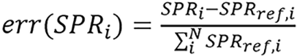
Equation (2) was used to compute ground truth SPR using I_w = 75 eV (mean excitation energy of water) at a proton energy of 200 MeV. The activation function used for all hidden layer was rectified linear unit and a linear function for final activation. The case which used patient data for training was referred to as ‘Unet(PT)’ and the second case which used custom computational phantoms for training was referred to as ‘Unet(PH)’. For Z-to-I conversion, 15 inserts were used for calibration to fit lnI = C₁Z² + C₂Z + C₃ for all Z; since only three materials were used in their simulation (i.e., air, water, and bone), all the materials below 1200 HU had very similar Z, hence, there was no need for a distinctive fit for these water-based materials. The relative error of each pixel was weighted according to its reference SPR to reflect its true impact on the overall range calculation because relative SPR errors from low density material (air) and high density material (bone) produce a substantially different impact on the overall range uncertainty. Relative error for pixel i[err(SPR_i)] was defined as

(39),

where N is the number of pixels in the population of interest.

The ME was defined as:

(40),

this is the same as the relative range error. Because ME shows systematic uncertainty only, the standard deviation was calculated to show a stochastic component from noise. Assuming a Gaussian distribution, the overall range uncertainty corresponding to 2σ or 95^th percentile was defined as:

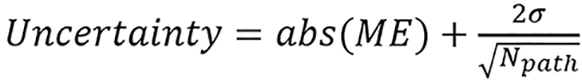(41),

where N_path is the number of pixels on an arbitrary proton path. N_path was chosen to be 100 to consider a typical case where the tumor is at a 10-cm depth with CT axial resolution as 1 mm/pixel. Some imaging techniques like masking and cropping were used in the study.

The result showed that both Unet(PT) and Unet(PH) seemed to produce a sharper SPR map than the conventional method. U-net may have learned how to sharpen edges even when it was trained with the phantom data. For HN test data, it showed that Unet(PH) consistently produced lower ME and standard deviation than the HS method. ME of the HS method was much higher than the prostrate case because the HN site has much higher air and bone content than the prostate, considering a much larger CT number variation due to the imaging artifacts. It was observed that U-net might have learnt how to better translate areas with transition of tissues from similar patient data for the case of Unet(PT) since the high error rates observed near the transition between air, soft, and bone tissues for both the HS method and Unet(PH) method was not observed with Unet(PT). U-net trained with computational phantoms reduced the SPR estimation uncertainty (95^th percentile) of the prostrate patient from 1.10% to 0.71%, and HN patient from 2.11% to 1.2%. U-net trained with patient images uncertainty values were 0.32% and 0.42% for prostate and HN patients, respectively, based on their report. These suggest that CNN has great potential to improve the accuracy of SPR estimation in proton therapy by incorporating individual patient geometry information compared to a conventional parametric model which was compared with the CNN. More experimental studies is needed for this approach. There is a need to decide if the computational time is worth the accuracy relative to parametric models. Further studies are needed to choose best hyperparameters for this kind of application, there might also be need to construct new activation functions based on tissue classification.

Machine learning approach

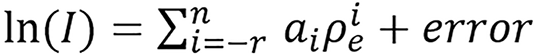
Chika[20] introduced a machine learning model and algorithm for computing I and SPR using relative electron density. This method provides a way of by passing Bethe or Bethe-Block equation. In his work he applied this model to BVM and H-S method by using the ρ_e computed by these methods to estimate SPR directly or first estimated I and used the Bethe-Block equation to estimate SPR. The model is stated below: SPR and mean excitation energy is empirically related to electron density by the relation:

(42),

where n ≥ 0, r ≥ 0 and T(SPR/I) is an invertible transformation of SPR or I.

The model was implemented for SPR as below:

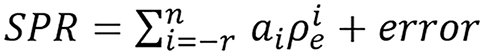(43),

where n ≥ 0, r ≥ 0 and T(SPR) = SPR. We will follow the notation SPR_r,n and present simple continuous and piece-wise functions. One of the interesting thing about the model was that it was able to get a good continuous fit for all the 33 human tissues (with total modeling RMSE as low as 0.31% and total testing RMSE of 0.71% as presented in Table 1) used without any tissue grouping, the continuous models presented are:

Table 1 Stopping power ratio training and testing root mean square errors (%) using reference ρ_e as presented in Chika[20].

SPR training RMSE (%)	Total	Lung	Soft	Bone	Testing RMSE (%)	Total	Soft	Bone
SPR1,1 continuous	0.32	0.70	0.35	0.13		0.73	0.80	0.62
SPR1,1 piece-wise	0.22	0.02	0.27	0.04		0.92	1.09	0.61
SPR0,3 continuous	0.31	0.14	0.38	0.07		0.71	0.77	0.62
Kanematsu	2.03	0.00	2.08	2.04		1.77	1.80	1.63

Citation: Chika CE. Estimation of Proton Stopping Power Ratio and Mean Excitation Energy Using Electron Density and Its Applications via Machine Learning Approach. J Med Phys 2024; 49: 155-166. Copyright© The Authors 2024. Published by Wolters Kluwer Medknow Publications. This article is available under the terms of the Creative Commons Attribution-NonCommercial-ShareAlike License (CC BY-NC-SA), which permits non-commercial use, distribution and reproduction in any medium, provided the original work is properly cited. Permission only needs to be obtained for commercial use. RMSE: Root mean square error; SPR: Stopping power ratio.

(44),

and

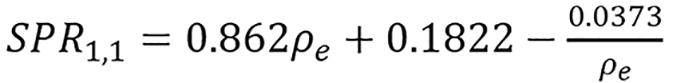(45),

shown in Figure 1.

Figure 1 This is the modeling plot of SPR_0,3 and SPR_1,1 (shows the relationship between the actual stopping power ratio data and the proposed model). The left figure is for SPR_0,3 and the right figure is for SPR_1,1. The stopping power ratio is plotted against the relative electron density on the graph. The small circles represent the actual value for the tissues and the line represents the model estimates. Citation: Chika CE. Estimation of Proton Stopping Power Ratio and Mean Excitation Energy Using Electron Density and Its Applications via Machine Learning Approach. J Med Phys 2024; 49: 155-166. Copyright© The Authors 2024. Published by Wolters Kluwer Medknow Publications. This article is available under the terms of the Creative Commons Attribution-NonCommercial-ShareAlike License (CC BY-NC-SA), which permits non-commercial use, distribution and reproduction in any medium, provided the original work is properly cited. Permission only needs to be obtained for commercial use. SPR: Stopping power ratio.

Other piece-wise version of the model was presented as an example which gave good result (with total modeling RMSE 0.22% and total testing RMSE of 0.92% as presented in Table 1). The examples were compared with the one proposed by Kanematsu et al[43] which is also a subset of the presented model. For the piece-wise examples, the tissues were classified into lung tissue, soft tissue and bone tissue. The comparison is presented in the Table 1. Similarly, examples of the model for estimating I was presented:

(46),

where n ≥ 0, r ≥ 0, preferably n = 2k, k ≥ 0, and T(I) = ln(I). Just as above he followed the notation I_r,n and presented two examples.

Continuous models:

(47).

Piece-wise model:

(48).

These were applied to the ρ_e computed using BVM and H-S method. Monochromatic attenuation at effective energy was used for the computation. The SPR computed using different mean excitation energies estimated via different approaches and the SPR estimated directly from the ρ_e were compared as presented in Table 2. Other I values used for comparison were computed using equation (8) and (9).

Table 2 Stopping power ratio training and testing root mean square error (%) using estimated ρ_e as presented in Chika[20].

SPR training RMSE (%)	Total	Lung	Soft	Bone	Testing RMSE (%)	Total	Soft	Bone
BVM SPR from I1,0	0.26	0.14	0.32	0.06		0.86	0.99	0.63
BVM SPR1,1	0.23	0.07	0.28	0.05		0.98	1.18	0.61
BVM SPR from Ifc	0.29	-0.09	0.31	0.28		1.59	0.61	2.36
BVM SPR from Irc	0.25	0.09	0.30	0.13		1.54	0.61	2.27
H-S SPR from I1,0	0.98	0.94	1.00	0.95		1.40	1.45	1.33
H-S SPR1,1	0.22	0.01	0.27	0.05		0.97	1.15	0.63
H-S Method	0.39	0.28	0.41	0.35		0.85	0.91	0.77

Citation: Chika CE. Estimation of Proton Stopping Power Ratio and Mean Excitation Energy Using Electron Density and Its Applications via Machine Learning Approach. J Med Phys 2024; 49: 155-166. Copyright© The Authors 2024. Published by Wolters Kluwer Medknow Publications. This article is available under the terms of the Creative Commons Attribution-NonCommercial-ShareAlike License (CC BY-NC-SA), which permits non-commercial use, distribution and reproduction in any medium, provided the original work is properly cited. Permission only needs to be obtained for commercial use. SPR: Stopping power ratio; RMSE: Root mean square error; BVM: Basis vector method; H-S: Hunemohr’s and Saito.

A total of 33 human biological tissues[3] were used as training data and 12 Gammex inserts as testing data. It was found that the ME for the presented examples of the model were close to zero indicating that the model estimation has low bias. Also, a machine learning algorithm was presented. Given ρ_e data: (1) Formulate the models; (2) Try different combination of r and n for the proposed model; (3) Check their training and testing error; and (4) Choose the optimal model for your data. More studies are required for experimental and clinical implementation. Studies which include more uncertainties especially in estimating ρ_e needs to be carried out to see how it propagates to the model estimations. More ways of improving the model can be considered like continuity between grouped tissue or the whole tissues. This model has the potential of estimating other parameters other than I and SPR which needs to be investigated.

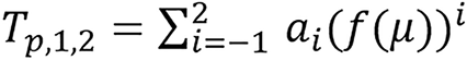
Chika[21] introduced a new image domain approach of estimating radiation parameters on image domain. It involves using machine learning model and algorithm to estimate the parameters with CT images. The model example was presented for estimating four parameters which include relative electron density (ρ_e), effective atomic number (Z), mean excitation energy (I) and SPR. We are going to be focusing on the SPR estimation on this paper. Example of equation (23) considered is

.

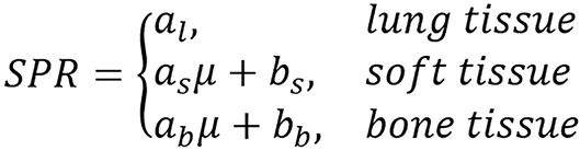
The examples considered for SPR are:

,

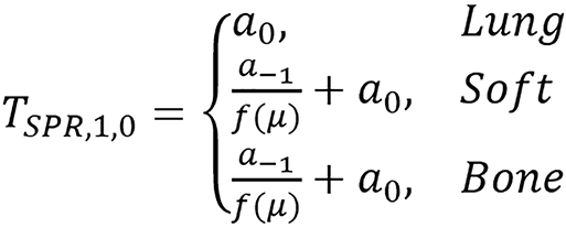and

.

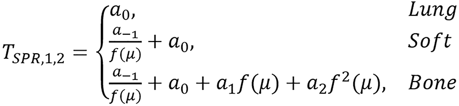The tissues were grouped into three (3) which are lung, soft and bone tissues. To improve the performance, further grouping was carried out which involves grouping the soft tissues into two making it four groups represented in the Tables 3 and 4 as 4 groups (4g). The grouping is presented in Figure 2. Figure 3 shows different dual energy approach modeling error for individual tissues. It was found that the proposed method can give better estimates for SPR using polychromatic theoretical CT-number. This model was also found to be flexible to modify and improve using classification or fitting degree.

Figure 2 Tissue classification using f(μ). A: Four regions of classification (lung tissues if f_r ≤ 0.3, soft tissue 1 if 0.3 < f_r ≤ 1.02, soft tissue 2 if 1.02 < f_r ≤ 1.4, and bone tissue if f_r > 1.4); B: Three regions of classification (lung tissues if f_L ≤ 0.3, soft tissue if 0.3 < f_L ≤ 1.4, and bone tissue if f_L > 1.4). Citation: Chika CE. Machine Learning Approach and Model for Predicting Proton Stopping Power Ratio and Other Parameters Using Computed Tomography Images. J Med Phys 2024; 49: 519-530. Copyright© The Authors 2024. Published by Wolters Kluwer Medknow Publications. This article is available under the terms of the Creative Commons Attribution-NonCommercial-ShareAlike License (CC BY-NC-SA), which permits non-commercial use, distribution and reproduction in any medium, provided the original work is properly cited. Permission only needs to be obtained for commercial use.

Figure 3 Individual tissues stopping power ratio relative error for the presented dual energy methods as presented in Chika[21]. The relative stopping power ratio estimating error for each tissue is plotted against the reference (actual) stopping power ratio on the graph. This is plotted for different methods as shown in figure legend where f_r (μ)= μ_L/μ_H. Citation: Chika CE. Machine Learning Approach and Model for Predicting Proton Stopping Power Ratio and Other Parameters Using Computed Tomography Images. J Med Phys 2024; 49: 519-530. Copyright© The Authors 2024. Published by Wolters Kluwer Medknow Publications. This article is available under the terms of the Creative Commons Attribution-NonCommercial-ShareAlike License (CC BY-NC-SA), which permits non-commercial use, distribution and reproduction in any medium, provided the original work is properly cited. Permission only needs to be obtained for commercial use. SPR: Stopping power ratio.

Table 3 Stopping power ratio modeling and testing root mean square (%) using computed tomography number as presented in Chika[21].

SPR training RMSE (%)	Total	Lung	Soft	Bone	Testing RMSE (%)	Total	Soft	Bone
TSPR,1,0;fr(μ)	1.78	0.04	0.58	2.98		4.72	4.80	4.61
TSPR,1,2;fr(μ)	0.49	0.04	0.58	0.26		5.87	4.82	7.08
TSPR,1,2;fm(μ)	1.04	0.03	1.14	0.87		3.89	3.07	4.80
TSPR,1,2;fL(μ)	0.85	0.00	1.00	0.53		3.14	3.28	3.27
Stochiometric	0.86	0.01	1.00	0.56		3.39	3.35	3.44
Taasti	0.60	0.01	0.22	1.00		6.77	7.19	6.14
H-S method	5.10	0.45	3.42	7.46		4.51	4.47	4.57
TSPR,1,2;fr(μ)4g	0.38	0.04	0.44	0.26		5.87	4.82	7.08

Citation: Chika CE. Machine Learning Approach and Model for Predicting Proton Stopping Power Ratio and Other Parameters Using Computed Tomography Images. J Med Phys 2024; 49: 519-530. Copyright© The Authors 2024. Published by Wolters Kluwer Medknow Publications. This article is available under the terms of the Creative Commons Attribution-NonCommercial-ShareAlike License (CC BY-NC-SA), which permits non-commercial use, distribution and reproduction in any medium, provided the original work is properly cited. Permission only needs to be obtained for commercial use. SPR: Stopping power ratio; RMSE: Root mean square; H-S method: Hunemohr’s and Saito model.

Table 4 Stopping power ratio modeling and testing mean error (%) using computed tomography number as presented in Chika[21].

SPR training ME(%)	Total	Lung	Soft	Bone	SPR testing ME(%)	Total	Soft	Bone
TSPR,1,0;fr(μ)	0.28	0.04	0.01	0.84		0.63	1.02	0.09
TSPR,1,2;fr(μ)	0.00	0.04	0.00	0.00		-0.05	1.06	-1.62
TSPR,1,2;fm(μ)	-0.09	-0.03	-0.02	-0.24		-2.08	-1.48	-2.92
TSPR,1,2;fL(μ)	0.00	0.00	-0.01	0.02		-1.04	-0.85	-1.30
Stochiometric	-0.01	-0.01	-0.01	-0.01		-1.15	-0.93	-1.46
Taasti	-0.02	-0.01	-0.01	-0.03		2.19	2.95	1.14
H-S method	0.17	0.45	2.25	-3.84		-0.23	2.66	-4.28
TSPR,1,2;fr(μ)4g	0.00	0.04	0.00	0.00		-0.31	0.62	-1.62

Citation: Chika CE. Machine Learning Approach and Model for Predicting Proton Stopping Power Ratio and Other Parameters Using Computed Tomography Images. J Med Phys 2024; 49: 519-530. Copyright© The Authors 2024. Published by Wolters Kluwer Medknow Publications. This article is available under the terms of the Creative Commons Attribution-NonCommercial-ShareAlike License (CC BY-NC-SA), which permits non-commercial use, distribution and reproduction in any medium, provided the original work is properly cited. Permission only needs to be obtained for commercial use. SPR: Stopping power ratio; ME: Mean error; H-S method: Hunemohr’s and Saito model.

Machine learning algorithm (modified for SPR) was also given as follows: (1) Given CT image data; (2) Compute μ; (3) Check empirical relationship between SPR and μ; (4) Construct f_μ; (5) Formulate T_SPR; (6) Classify the tissues; (7) Estimate the constant of combinations a_i; (8) Check the modeling and testing error; and (9) Repeat iv-viii until optimal acceptable error is reached given more priority to testing error.

Generalized version of the model was also stated as: Given a radiological parameter p related to the attenuation coefficient μ and some other parameters p’, there exist transformations/maps T_(p) and f(μ) such that

(49),

n ≥ 0, j ≥ 0 and p = T^-1[T(p)], a_i∈R, where μ = (μ₁, μ₂, μ₃, …, μ_n) for n-energies with at least one low energy, p’ = (p’₁, p’₂, p’₃, …, p’_k) for K-known parameters and err is an acceptable error. In the original paper T_SPR1,0 is denoted as T_SPR1,1 though this does not affect the meaning since the provided table of parameters for this case assigned zeros to all a₁, i.e., a₁= 0. Also, equations (23) and (49) are written as

and

respectively for the model; this includes the constant, a_i, inside the parenthesis before the exponent. Though this does not affect the meaning of the model since it can be simplified and substituted with another constant, for example,

,

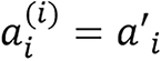the more appropriate representation is

and

respectively, i.e., the constant (a_i) is not inside the parenthesis.

Example:

.

From Figure 3, T_SPR,1,2;f_r(μ) and T_SPR,1,2;f_r(μ)4g relative error values are closer to the line representing zero error, showing that the individual tissues error estimates are very low. Therefore, this provides a better estimate of SPR for the presented individual tissues compared to the other presented methods. Table 3 shows that T_SPR,1,2;f_r(μ) was able to achieve the lowest total testing RMSE (3.14%) and lowest testing RMSE (3.27%) for bone, T_SPR,1,2;f_r(μ) has the lowest RMSE (3.07%) for soft tissue, T_SPR,1,2;f_r(μ)4g achieved the total modeling RMSE (0.38%); though, Taasti method achieved the lowest modeling RMSE (0.22%) for soft tissue, this moved to 7.19% in testing which shows higher sensitivity to change in CT number compared to other presented methods. This implies that this proposed model is not just accurate but also more robust compared to other presented methods based on the used data. Table 4 shows that the modeling ME for the presented methods are all closer to zero showing low bias in modeling.

There are still many studies to be conducted on this like the uncertainty study, experimental and clinical study, model continuity study and ways of improvement. Some further studies have been done on uncertainty and comparison, Li et al[9] presented more comprehensive uncertainty study on dual energy approach using H-S method and Bourque’s method where they analyzed the factors contributing to DECT based method and found that DECT approach can reduce the overall range uncertainty to approximately 2.2% (2σ) in clinical scenarios. Vilches-Freixas et al[44] carried out comparison between one projection domain method and three image domain method for DECT approach and found that projection domain method gives slightly more accurate result. As it is further stated in Yang et al[2], Bazalova et al[27] carried out DECT study for calculating Z_eff and ρ_e using measured CT number with T-S method where the largest impact on the DECT calculation was caused by beam hardening effect, resulting to substantial underestimation of ρ_e for materials with high Z_eff. Image noise also has a large impact on the DECT calculation.There are several ways to reduce random noise which one is increasing the pixel size since high resolution is not required for treatment planning. Some other techniques like convolution techniques presented by Chidiebere and Chika[45] can be used to improve or maintain image quality while computing SPR. The DECT method will be more susceptible to patient movement between two image scans and the parameters used in image reconstruction can have an impact on the DECT calculation. When CT artifacts such as beam hardening, scatter, noise, etc. are considered, theorectical high accuracy achieved in DECT method may not be achievable in practical situations like clinical settings. Since RMSE remained below 1% for most cases using the DECT method, this implies that the DECT method might be more suitable for measuring patient-specific tissue compositions to improve the accuracy of treatment planning for charged particle therapy[2].

CONCLUSION

The DECT approach demonstrates significant promise, as evidenced by multiple studies reviewed in this paper. Both image and projection domain methods have their advantages. This review discusses the major dual energy methods currently under active investigation. Based on good performance of this approach especially in its robustness to uncertainty, further studies are recommended to facilitate its quick clinical implementation. We recommend detailed studies on the practical uncertainties of these methods, as well as further experimental studies, validation in clinical trials, and projection domain research to enhance imaging quality.