Machine learning-based nomogram for predicting depressive symptoms in women: A cross-sectional study in Guangdong Province, China

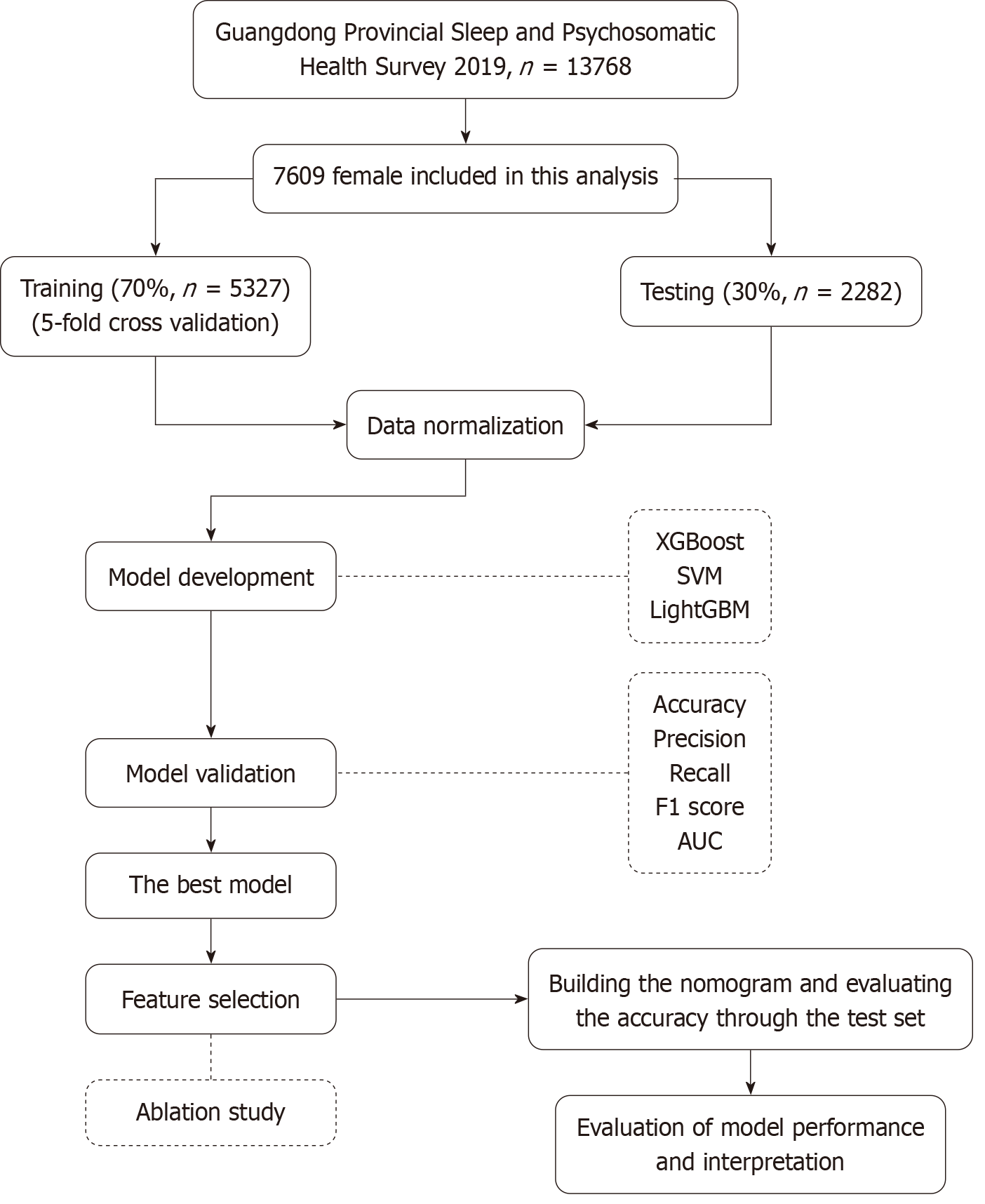
Figure 1 The flow diagram of data processing and model building process. XGBoost: Extreme gradient boosting; SVM: Support vector machine; LightGBM: Light gradient boosting machine; AUC: Area under the curve.

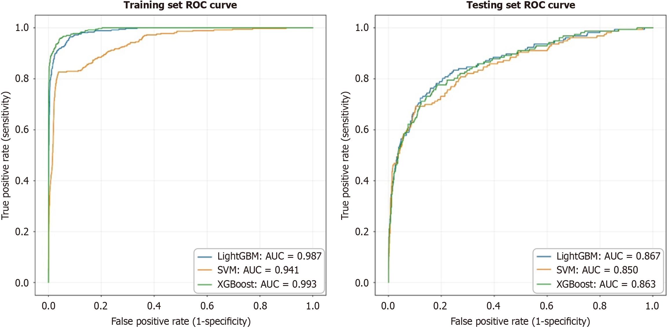
Figure 2 The receiver operating characteristic curve of all models. ROC: Receiver operating characteristic; XGBoost: Extreme gradient boosting; SVM: Support vector machine; LightGBM: Light gradient boosting machine; AUC: Area under the curve.

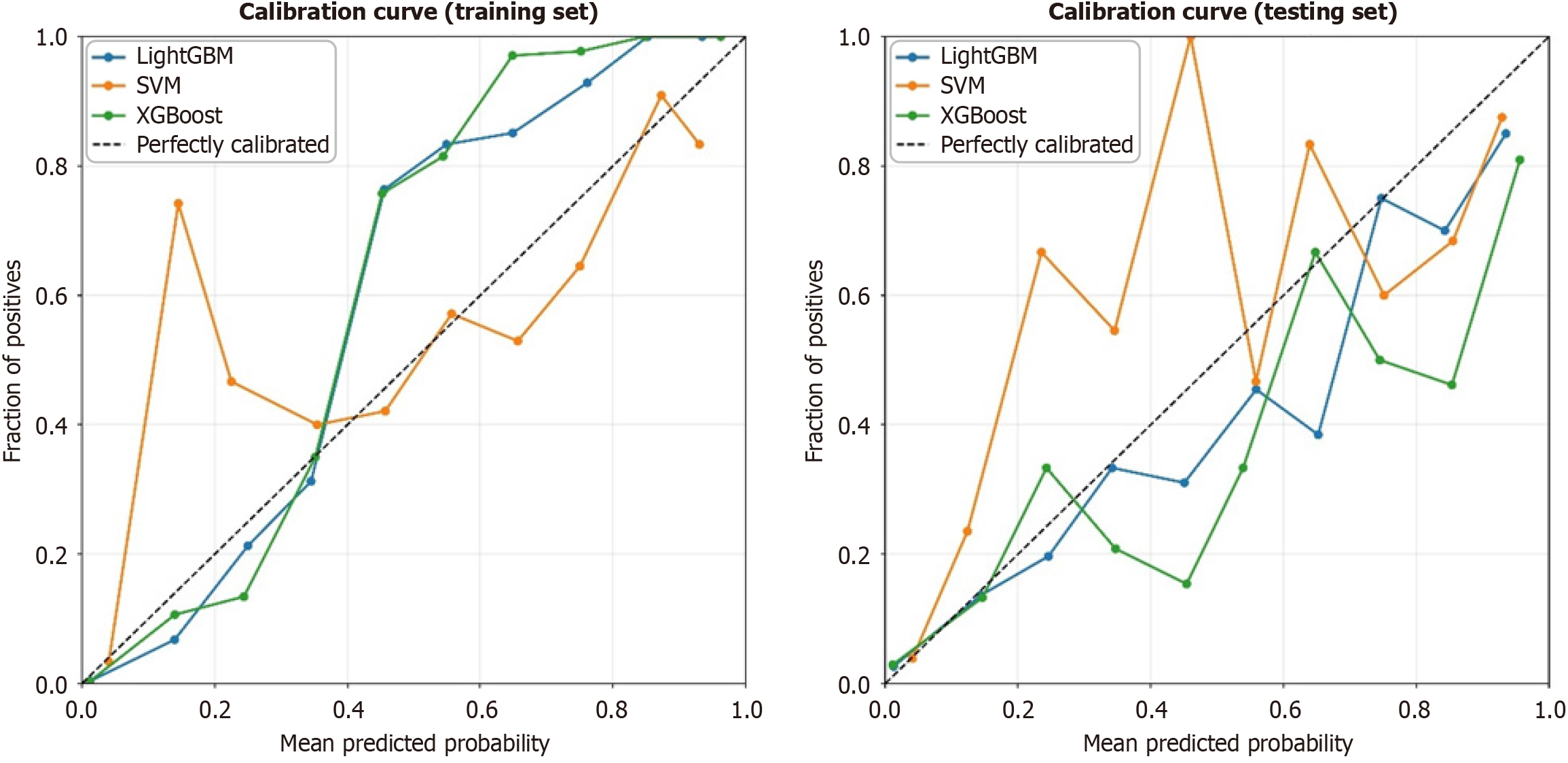
Figure 3 Calibration curve of all models. XGBoost: Extreme gradient boosting; SVM: Support vector machine; LightGBM: Light gradient boosting machine.

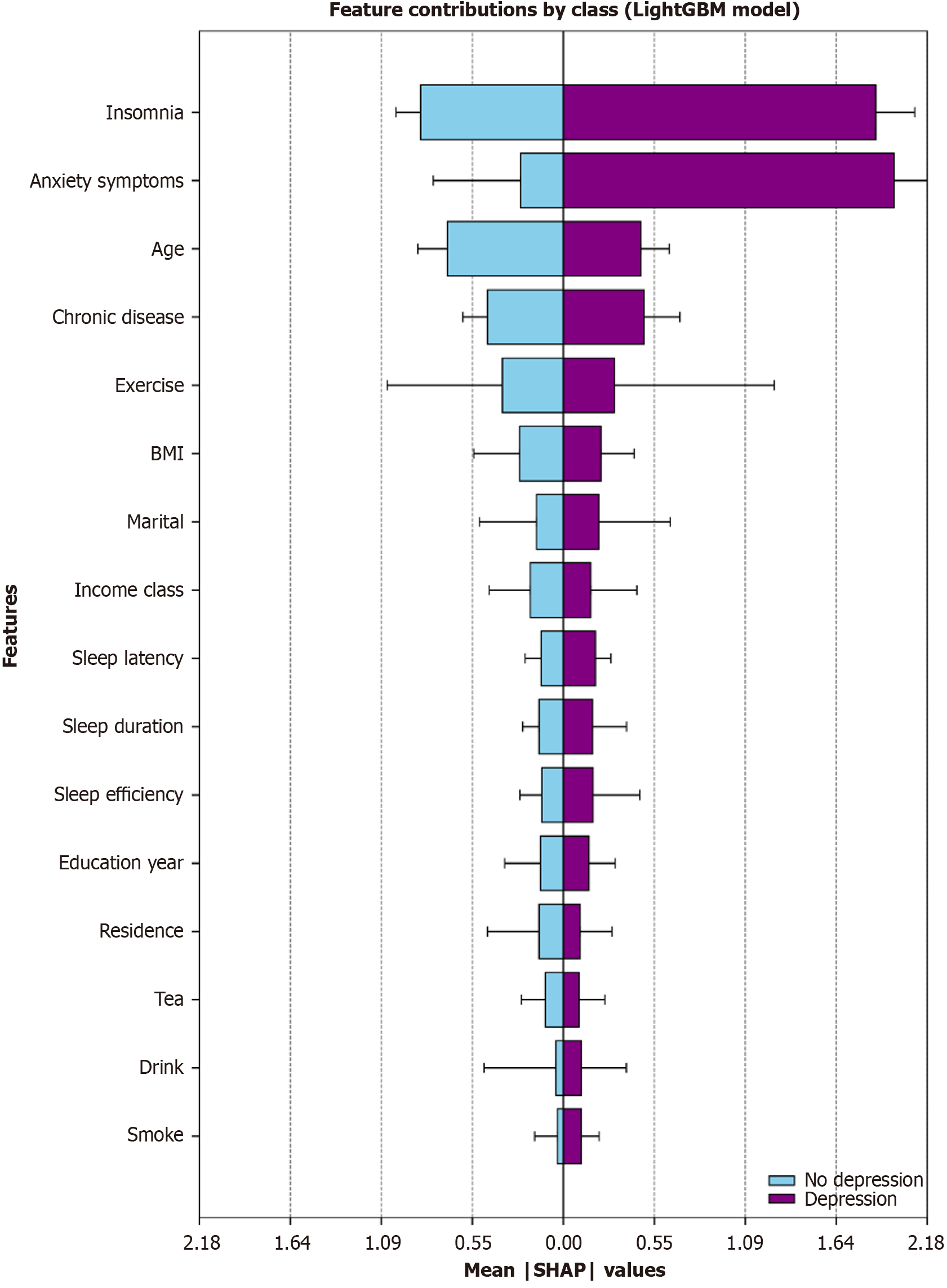
Figure 4 Feature contributions by class using SHapley Additive exPlanations values. LightGBM: Light gradient boosting machine; SHAP: SHapley Additive exPlanations.

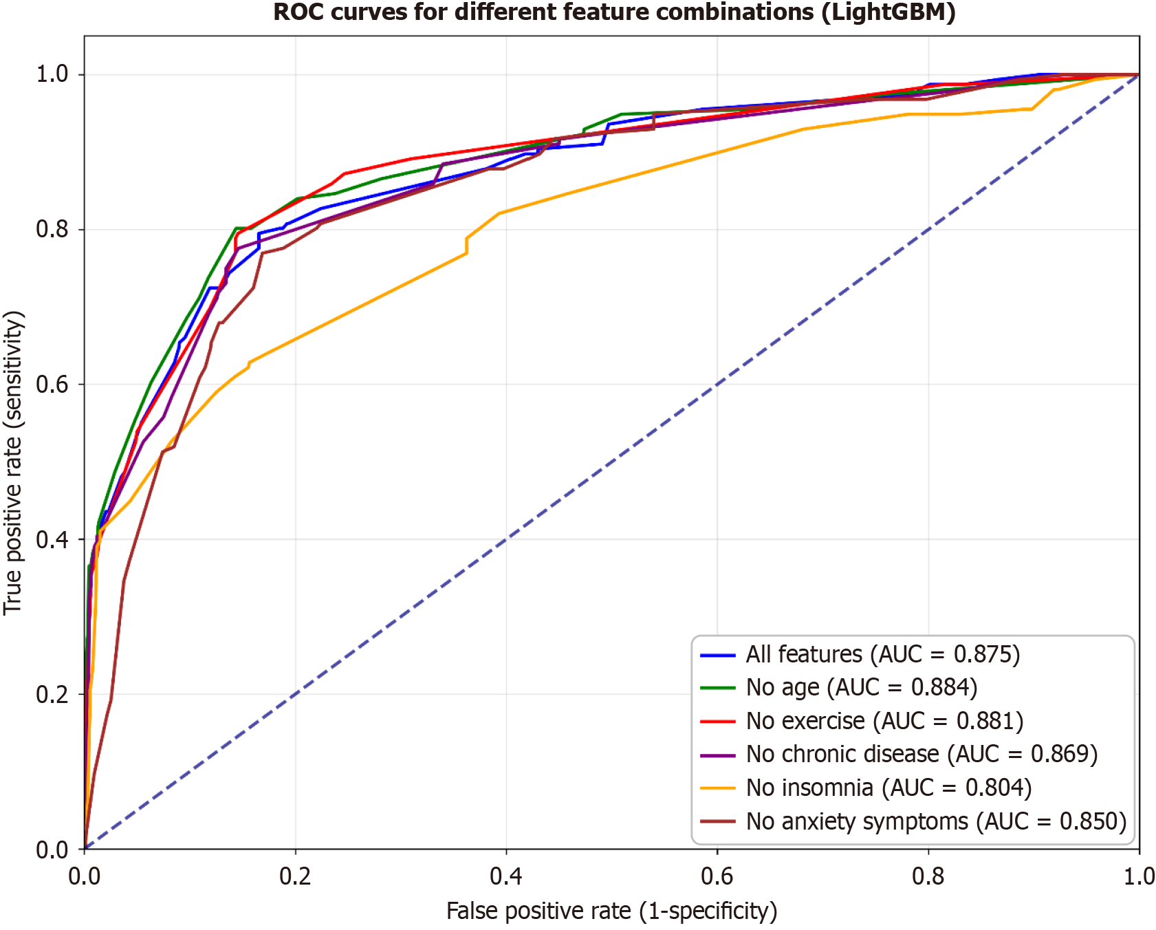
Figure 5 Ablation study on key features using the receiver operating characteristic curve. LightGBM: Light gradient boosting machine; ROC: Receiver operating characteristic; AUC: Area under the curve.

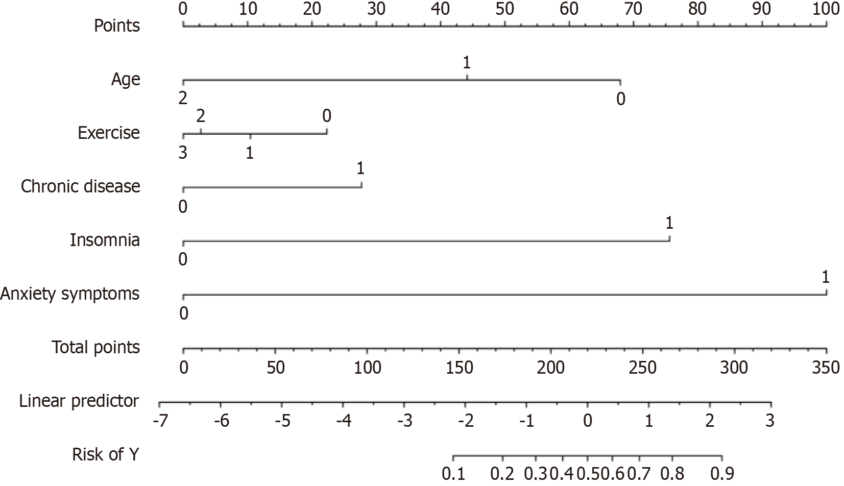
Figure 6 Nomogram for predicting the risk of depression based on insomnia, anxiety symptoms, chronic disease, exercise, and age. The total points are used to calculate the linear predictor and risk probability.

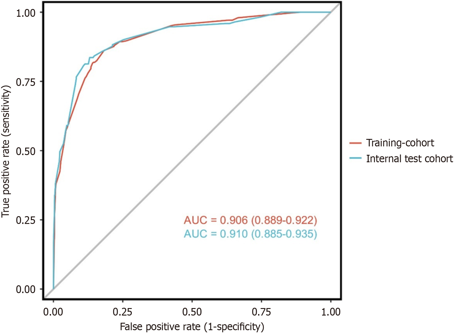
Figure 7 The receiver operating characteristic curves for the predictive model in the training and internal test cohorts. AUC: Area under the curve.

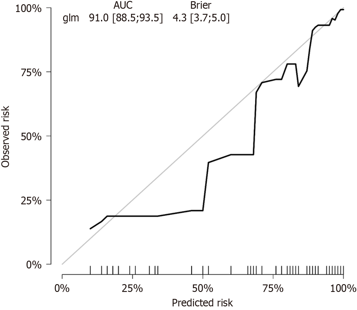
Figure 8 Calibration plot for the logistic regression model. The plot shows the relationship between predicted and observed risks. AUC: Area under the curve.

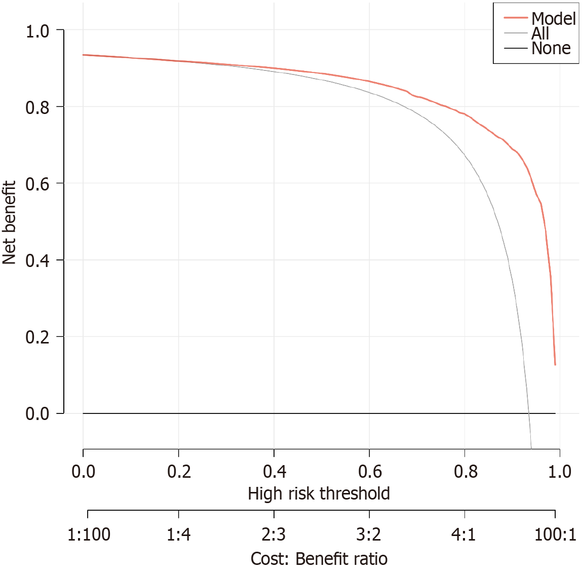
Figure 9 Decision curve analysis for the predictive model. The plot shows the net benefit of the model across varying thresholds of high risk, compared to strategies of treating all patients or treating none.