Published online Jun 26, 2014. doi: 10.5662/wjm.v4.i2.109
Revised: February 13, 2014
Accepted: April 16, 2014
Published online: June 26, 2014
Processing time: 279 Days and 17.8 Hours
AIM: To present statistical tools to model and optimize the cost of a randomized clinical trial as a function of the stringency of patient inclusion criteria.
METHODS: We consider a two treatment, dichotomous outcome trial that includes a proportion of patients who are strong responders to the tested intervention. Patients are screened for inclusion using an arbitrary number of test results that are combined into an aggregate suitability score. The screening score is regarded as a diagnostic test for the responsive phenotype, having a specific cutoff value for inclusion and a particular sensitivity and specificity. The cutoff is a measure of stringency of inclusion criteria. Total cost is modeled as a function of the cutoff value, number of patients screened, the number of patients included, the case occurrence rate, response probabilities for control and experimental treatments, and the trial duration required to produce a statistically significant result with a specified power. Regression methods are developed to estimate relevant model parameters from pilot data in an adaptive trial design.
RESULTS: The patient numbers and total cost are strongly related to the choice of the cutoff for inclusion. Clear cost minimums exist between 5.6 and 6.1 on a representative 10-point scale of exclusiveness. Potential cost savings for typical trial scenarios range in millions of dollars. As the response rate for controls approaches 50%, the proper choice of inclusion criteria can mean the difference between a successful trial and a failed trial.
CONCLUSION: Early formal estimation of optimal inclusion criteria allows planning of clinical trials to avoid high costs, excessive delays, and moral hazards of Type II errors.
Core tip: This paper presents statistical tools to model and optimize the cost of a randomized clinical trial as a function of the stringency of patient inclusion criteria. The patient numbers and total cost are strongly related to the choice of the cutoff for inclusion. Clear cost minimums exist for many realistic scenarios. Potential cost savings for typical trial scenarios range in millions of dollars. Early formal estimation of optimal inclusion criteria allows planning of clinical trials to avoid high costs, excessive delays, and moral hazards of type II errors.
- Citation: Babbs CF. Choosing inclusion criteria that minimize the time and cost of clinical trials. World J Methodol 2014; 4(2): 109-122
- URL: https://www.wjgnet.com/2222-0682/full/v4/i2/109.htm
- DOI: https://dx.doi.org/10.5662/wjm.v4.i2.109
Clinical trials are too costly and take too long to complete. High costs of clinical trials add significantly to the ultimate costs of new medicines and medical devices. Delay in completion of a trial due to inefficient trial design can postpone, sometimes indefinitely, the transfer of promising new therapies from bench to bedside. Assuming that a true positive treatment effect exists, strategies are needed for finding the most direct route to a statistically significant result using the smallest numbers of patients.
When a genuinely responsive subset of patients is diluted with many patients who are genetically or physiologically ill suited to respond to a new experimental treatment, the numbers of patients that must be studied to disprove the null hypothesis increases dramatically. Type II errors in statistical inference (accepting the null hypothesis when it is false) can arise, and a useful drug, device, or procedure, which could have benefited some classes of patients, may be lost to further development. This situation is especially likely when only a fraction of patients in the treatment group respond well to the tested intervention, and when the control or comparison group is treated with a known, effective standard therapy, as is often done for ethical reasons. In this situation patient selection criteria are crucial.
An era of personalized medicine is emerging in which novel biochemical markers will be found for the diagnosis of cancer and other diseases[1]. When a genetic variation is linked to a specific drug effect, it becomes a biomarker that helps predict how an individual will react to a drug[2]. The treatment of cancer, in particular, is moving towards the use of more specific therapies that are targeted to each tumor type. To facilitate this shift, tests are being developed to identify those individuals who are most likely to benefit from particular treatments on the basis of the genes expressed by their tumors[3]. Such biomarkers may identify patients who will experience the most drug benefit and fewest side effects. In this setting innovative thinking about clinical trial design is needed to increase the proportion of patients receiving the best individual treatment, and to complete the trial more rapidly with fewer patients. There is also an ethical dimension to more efficient trial design: increasing the probability of a patient’s being allocated to a successful treatment. With targeted, personalized therapy the study patients do not have to pay a high price for the benefit of future patients[4]. The challenge moving forward is to identify optimal trial design in a population with known biomarker levels, based upon screening data, and to identify the optimal allocation of patients to treatment groups, based upon mathematical and computer simulation of the trial.
Here we consider a paradigm in which either a phase II trial data or an adaptive trial design provides pilot data describing responsiveness to the tested intervention in various types of patients. We consider the planning of a follow-on phase III trial, in particular a two-treatment randomized clinical trial, including a control group and an experimental group and having a dichotomous end point such as response vs non-response to treatment. The definition of response is at the discretion of the investigator and is based on clinically desirable outcomes. Examples include disease free survival from cancer for a period of one year, induction of a state of clinical remission in leukemia, or resuscitation from cardiac arrest with a measurable pulse and blood pressure. The primary endpoints of the future trial are the proportions of patients that respond in the experimental group and in the control group.
The goal of the present research is to create a formal mathematical model of the planned randomized trial that will allow one to define and predict an optimal set of inclusion criteria. Such criteria would screen out non-responsive patient types and achieve a statistically significant result with the smallest number of patients and the lowest overall cost in both time and resources. In such a trial patients who are prospective candidates having an appropriate diagnosis would be screened according a list of possible metrics, such as age, tumor stage, or biomarker level. The screening metrics, here denoted x1, x2, ¡, etc. are combined mathematically by a classifier function, F (x1, x2, ¡), based on pilot data to obtain a single overall score, x = F (x1, x2, ¡), which is a predictor of successful response. Future patients for whom x equals or exceeds a cutoff value xc will be included in the trial, and patients for whom x < xc will be excluded. Combinations of x1, x2, ¡, etc. yielding values of x ≥ xc constitute the inclusion criteria for the study. The questions addressed by this paper are how to define a satisfactory classifier F (x1, x2, ¡) and how to best choose xc to produce a statistically significant positive result with minimal time and cost, assuming an alternative hypothesis of a true treatment effect.
To help predict the most favorable inclusion criteria, it is helpful to regard the screening process and the function F (x1, x2, ¡) as a diagnostic test, for which the concepts of sensitivity and specificity apply. This paper demonstrates how one can use data from a one-armed phase II study or early-stage pilot data from an adaptive trail design to create a suitable classifier F (x1, x2, ¡) for discriminating responders from non-responders and also to predict the best cutoff, xc, for inclusion of future patients.
Suppose that a planned, two-arm, randomized clinical trial begins with evaluation of N possible candidates having a standard clinical diagnosis such as biopsy proven carcinoma of the breast. Suppose further that this population is heterogeneous in the sense that a proportion, q, of the patients are biologically well suited to respond to the experimental treatment (call them type 1 patients) having success probability π1 ≈ 1, and the remaining proportion, 1 - q, of the patients are biologically ill suited to respond to the experimental treatment (call them type 2 patients) having success probability π2 ≈ 0. It is normally not possible to predict in advance which patients will respond, but one can try to establish favorable inclusion criteria based on certain screening data. These data may be a simple as age, gender, and stage of disease or may include sophisticated measures of biomarkers.
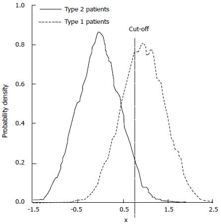
If the screening procedure had 100% sensitivity and 100% specificity for detecting guaranteed responsive type 1 individuals, who are very likely to respond to the new therapy, then the inclusion decision would be trivial: only type 1s would be included. In the more common situation potential good responders are difficult to identify, and a battery of imperfect metrics is employed. Suppose that such a battery of tests exists and that the test results x1, x2, etc. are combined in a single overall suitability test score, x = F (x1, x2, ¡). Type 1 and type 2 patients are likely to be distributed along the x-scale as shown in Figure 1, with significant overlap. Overlap of the distributions leads to meaningful fractions of false positive evaluations and false negative evaluations for the presence of the treatment responsive phenotype, given any chosen cutoff, xc , for entry into the study.
In this sense we can regard the process of patient selection as a “diagnostic test”, for which the concepts of sensitivity (true positive fraction, ftp) and specificity (true negative fraction, ftn) apply. The false positive fraction, ffp = 1 - ftn. If q is the fraction of type 1 individuals in the initial population of N patients and if 1 - q is the fraction of type 2 individuals, then Nqftp type 1s and N (1 - q )ffp type 2s will be selected for inclusion in the trial. As the cutoff xc, is raised, the entry criteria become more strict, specificity for the responsive type 1 phenotype increases, but sensitivity decreases. Some potential good responders are excluded, and the overall study size is decreased, reducing its statistical power. In the limiting case over-strict inclusion criteria will reject nearly all patients. The time required to find perfect candidates will be excessive, and study numbers will be small. On the other hand, as the cutoff xc, is reduced, the entry criteria become more loose. Sensitivity increases, but specificity decreases. The population of patients included in the trail is diluted with more and more non-responding type 2 patients. If q is small, the time and cost required to establish a significant treatment effect may become prohibitive.
It is reasonable to use N, the number of candidates initially considered for the trial before the screening process, as a measure of the cost of screening and also as one measure of the time required to complete the study. (If extensive long term follow-up is required, a constant plus N can be substituted.) It is also reasonable to use N’ = Nqftp + N (1 - q )ffp , the actual number of patients enrolled in the study, as a measure of the cost of treating and managing the patients over the course of the trial.
The mathematical treatment that follows includes several parts with the following objectives: (1) to create a formal mathematical model of the proposed randomized trial, given preliminary screening and outcome data; (2) to illustrate how such a model can be used to estimate the probability distribution of a test statistic describing the outcome of the trial; (3) to exercise the model to predict the number, N, of patients that must be screened and the number, N’, of patients that must be included to reject the null hypothesis with a specified power, given the sensitivity and specificity of the screening process; (4) to characterize the sensitivity and specificity of the screening process as a receiver operating characteristic (ROC) curve; and (5) to compute the cost of the trial as a function of N and N’ and to demonstrate how the cost varies as a function of the stringency of the inclusion criteria, based on the cutoff xc, and in turn to determine if there is a “best” cutoff, xc, for which a cost function of N and N’ is minimized.
Suppose, as before, that N patients are available to be screened for inclusion in a future randomized clinical trial comparing experimental and control groups. The end point of the trial is dichotomous. A fraction, 0 < q < 1, of patients will respond well to the experimental treatment based on their genetics or physiology. Denote these good responding individuals as type 1 patients and remainder of non-responding individuals as type 2 patients. A screening procedure is performed having overall sensitivity ftp, specificity ftn, and false positive fraction ffp = 1 - ftn . After screening and evaluation n = ftpNq type 1 patients and m = ffp N(1 - q) type 2 patients will be selected for inclusion in the trial. These selected patients will be randomized into control and treatment groups, which for generality need not be equal, having α (n + m) patients in the experimental group and (1 - α)(n + m) patients in the control group for 0 < α < 1.
Consider a model in which the probability of favorable outcome after the experimental treatment among type 1s is π1 = 1, and the probability of favorable outcome after the experimental treatment among type 2s is π2 = 0. To allow for the possibility that the type 1s and type 2s may also respond differently after the control treatment, let the probability of favorable outcome after the control treatment among type 1s be π3 and the probability of favorable outcome to the control treatment among type 2s be π4 (Numerical values for π3 and π4 will be estimated from pilot data or published literature as described later). The expected outcome of the trial is shown in Table 1, showing the mean number of observed responders (successful outcomes) in each group.
| Experimental group | Control group | |
| Number of successes (responses) | α (nπ1 + mπ2) | (1 - α) (nπ3 + mπ4) |
| Total | α (n + m) | (1 - α) (n + m) |
Let us use the difference in proportion test for statistical inference for the purpose of predicting trial size and cost. (This choice in no way prevents the use of other statistical measures and tests of significance for reporting later results, including internal meta-analysis of the various stages[5,6]). The difference in the proportion of responders ∆p = pE - pC between experimental and control groups is computed and then divided by an estimate,
Math 10
, of the standard deviation, σ, of the difference of proportions to obtain a test statistic z = ∆p/
Math 11
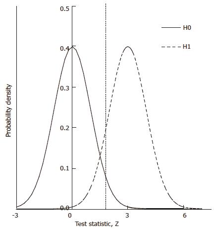
. Under the null hypothesis, H0, the expected value of the z-statistic is zero and the standard deviation of the z-statistic is 1, as shown by the thin curve in Figure 2.
To explore the predicted N required for a statistically significant study as a function of model parameters, we can compute the distribution of the test statistic, z, under the alternative hypothesis, H1, of a positive effect of experimental treatment. The form of this distribution, represented by the thick curve in Figure 2, is a function of model parameters, including probabilities π1, π2, π3, and π4, the number, N, of patients screened and the cutoff for patient inclusion. The distribution of z is characterized by its mean and variance, as follows.
From Table 1 the expected value, μ, of the difference in sampled proportions between the experimental and control groups is
μ = [n(π1 - π3) + m(π2 - π4)]/(n + m) (1a).
The variance of the difference in proportions is the sum of the variances of the independent sample proportions σ2 = σ2(pE) + σ2(pC). To find the variances note that the true population probabilities for responses in the experimental group and the control group are
πE = (nπ1 + mπ2)/(m + n)
and
πC = (nπ3 + mπ4)/(m + n) (1b).
Hence, using the standard formulas for the variances of binomial distributions[7],
σ2 (pE) = [πE(1 - πE)]/[α(n + m)]
and
σ2 (pC) = [πC(1 - πC)]/[(1 - α)(n + m)] (1c)
with
1-πE = (n + m - nπ1 - mπ2)/(n + m)
= [n (1 - π1) + m (1 - π2)]/(n + m)
and similarly for 1 - πC .
Under the null hypothesis of zero treatment effect compared to control, the expected value of pE - pC = 0, and the test statistic
Math 12
will have mean value
Math 13
and a standard deviation of one. That is, z will be distributed to good approximation as the standard normal distribution under H0.
Under the alternative hypothesis of an expected positive treatment effect the expected value, μ, of pE– pC will be greater than zero, and the test statistic, z, will have mean value,
Math 14
. The value of under H1 is related to the values of parameters (1a) through (1c) and and to the critical values for significance testing and the statistical power of the trial. For example, for P < 0.05 the critical value is 1.96, and for a power of 84%, that is an 84% probability of detecting a true effect as significant, then
Math 15
must be 1.0 standard deviation to the right of the cutoff in Figure 2, so that
Math 16
. To find the N and inclusion cutoff required to identify as statistically significant a particular treatment effect with a particular power we can explicitly evaluate
Math 17
in terms of model parameters. Then
Math 18
Knowing the target location of
Math 19
, one can estimate the statistical distribution of the results of the proposed trial, based upon the model parameters and the pilot screening and outcome data.
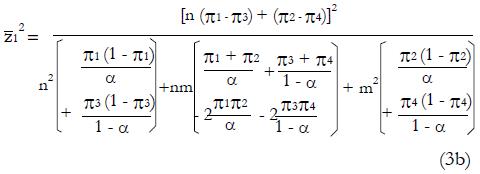
After squaring (3a), substituting expressions (1), and simplifying the algebra,
Math 20
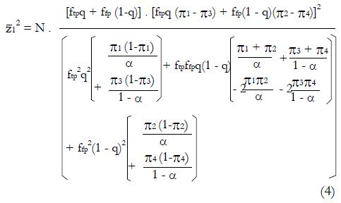
Then substituting n = ftpqN and m = ftpN(1 - q) gives,
Math 21
which can be solved for N as a function of model parameters ftp, ffp, q, zc, π1 through π4 , and the target power and level of significance represented by
Math 22
.
Expression (4) predicts N as a function of the proportion, q, of good responders in the population, the sensitivity and specificity of the screening procedure for inclusion into the study, and the effectiveness of the treatment in controls. Note since we use the square of
Math 23
to get N, the resulting N could be that for a significant positive result with pE > pC or a significant negative result with pC > pE. As expected, the required N becomes infinite, given the other parameters, when the null hypothesis is exactly true and the expected value of pE equals the expected value of pC.
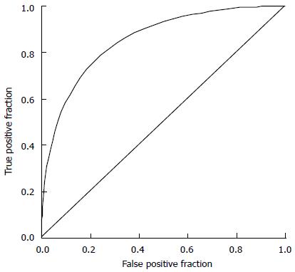
To explore the effects of more selective vs less selective inclusion criteria, one can examine paired combinations of true positive fractions and false positive fractions for a typical screening procedure as defined by a ROC curve. An ROC curve is a plot of ftp as a function of ffp in the unit square, as the cutoff value of decision variable, x, is gradually reduced from the maximum possible value of x toward the minimum possible value. A typical ROC curve is illustrated in Figure 3. Each point on the curve represents a realistic combination of ftp and ffp (sensitivity and 1- specificity) for a particular classifier used to distinguish type 1 vs type 2 patients.
In this context the ROC curve describes a family of cutoff values in the x-domain for partially overlapping distributions of good responding, type 1 patients and non-responding, type 2 patients. An ROC curve that is shifted upward and to the left indicates a better discriminating screening test. The ROC curve provides a useful mathematical model of stricter vs looser inclusion criteria for a clinical trial.
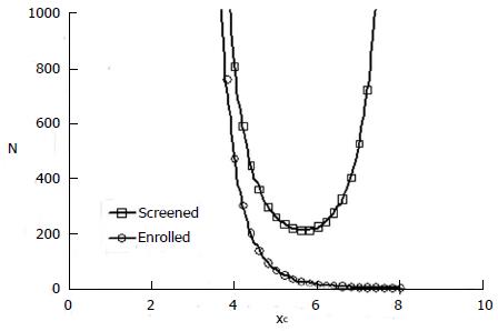
With this model one can explore the influence of inclusion criteria on the size and cost of the clinical trial. The top curve in Figure 4 is a representative plot of N from expression (4) as a function of cutoff value xc. N represents the number of patients screened in a hypothetical clinical trial with a statistically significant positive result (P = 0.05).
The number of patients actually enrolled in the trial after screening, according to the definitions of the model, is
N’ = n + m = ftpNq + ffpN(1 - q) (5).
This number is plotted as the bottom curve in Figure 4 for one hypothetical example.
In this example the mean composite screening score, xc, for responders is 5.5 and the standard deviation is 1. The mean composite screening score for non-responders is 4.0 with a standard deviation of 1. The ROC curve for this scenario is that of Figure 3. A value of cutoff xc < 2 means that all comers were included in the study. That is, there was no selection. A cutoff > 8 means that virtually all patients were excluded. In the mid range of inclusion criteria, there remains a strong effect of screening selectivity on the number of patients required to produce a significant result, given the alternative hypothesis. There is a clear optimal cutoff for patient selection near xc = 5.6 that minimizes the number of patients, N, with an initial diagnosis needed to produce a statistically significant positive result.
A total cost model is easily developed from the forgoing. The value of N as a function of ftp and ffp is a measure of the cost of screening, since all suitable patients must be screened. The value of N’ as a function of ftp and ffp is a measure of the cost for treatment and monitoring of enrolled patients, since more enrolled patients will require more personnel, facilities, coordination, data management, etc. The opportunity cost of delayed revenue from a successful new product and the opportunity cost of diversion of resources from other worthwhile projects are related to the duration of the trial.
Let c1 be the cost of screening per patient. Let c2 be the average cost of treatment per patient in both control and experimental groups. Let c3 be the opportunity cost per year in delay of marketing a successful drug or device, that is, the expected revenue divided by the duration of the study. Let r be the case rate, that is, the rate at which new cases appear for screening, and let t be the time required for follow up of a patient after entry into the study. In this case the total cost of the study is
Cost = c1N + c2N’ + c3(N/r + t). (6)
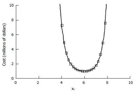
Additional cost terms can be added, if desired, such as performance site start-up costs, which would be related to N divided by the number of proposed sites. Figure 5 shows for the preceding example in Figure 4 the total cost calculation for the hypothetical cost constants given in the figure legend.
The anticipated cost of the study is strongly dependent on the stringency of the inclusion criteria. A low cost sweet spot exists for a narrow range of inclusion cutoff values in the range of 5.6 to 6.1 for this model. The result is consistent with qualitative experience that good results occur in a reasonable amount of time when patient selection is targeted and rigorous, but not so rigorous as to choke off the number of patients entering the trial who might benefit.
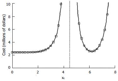
A particularly interesting situation arises when the average response probability for all patients given the experimental treatment, which is equal to q, is less than that for type 2 patients given the control treatment. In Figure 6 we have the situation in which π1 = 1.0 and π2 = 0, and q = 0.2, as before. However, we have π3 = π4 = 0.4. The experimental drug is much less effective than control treatment for type 2 patients. The cost projections include a vertical asymptote when the null hypothesis is exactly true, that is the expected value of pE equals the expected value of pC. To the right of the dashed line a significant positive effect, pE > pC, can be detected at the indicated cost. To the left of the dashed line a significant negative effect, pC > pE, can be detected. In such situations, which may be quite common in practice, choice of inclusion criteria could well make the difference between a futile study and a successful one. Thus the choice of inclusion criteria clearly can have large effects on the cost and success of a clinical trial.
The next sections develop methods to construct a classifier F(x1, x2, ¡ ) and to estimate the model parameters in an adaptive clinical trial, based on a phase II pilot data for treatment outcome and for screening variables, x1, x2, ¡etc. Such calculations would allow estimation of the optimal choice of inclusion criteria in a phase III trial for lowest cost and highest efficiency.
Model based prediction of optimal inclusion criteria requires the creation of an effective classifier to screen for type 1 patients based upon pilot data. Here we derive a relatively simple and effective linear classifier for combining an arbitrary number of screening variables, x1, x2, ¡ xk, to obtain a single overall predictor x = F(x1, x2, ¡ xk). Using the distributions of combined screening results, x, for responders and for non-responders to the experimental treatment, one can estimate the ROC curve for detection of good responding, type 1 patients. Here “responders” are those patients observed to have a successful outcome from the experimental treatment. “Non-responders” are those patients observed to have a poor outcome from the experimental treatment.
To create a classifier one must first examine screening data and outcomes in response to the experimental treatment in available preliminary data for all comers. The association between satisfactory response and possible predictors x1, x2, ¡ , such as age, sex, tumor stage, or biomarker level, can be judged by plotting the distributions of each variable for responders and non-responders. Continuous variables are dichotomized in a convenient way, using the joint median or a cutoff suggested by the shapes of the screening data distributions, for example, age < 50 years = 0 (young) and age ≥ 50 years = 1 (old). An apparent difference in the proportions of responders vs non-responders suggests that useful predictive information is captured by variable xi. Combining three or four features, xi , in different domains of anatomy and physiology will likely lead to more accurate prediction of response to therapy.
As shown in Appendix 1, a near optimal choice of a linear classifier function for k relatively independent or poorly correlated predictors, x1 , x2¡, xk, is
Math 24
where constant coefficients
Math 25
and subscript R indicates responders to the experimental treatment in the preliminary data set and subscript NR indicates non-responders.
For dichotomous variables
Math 26
the mean value is
Math 27
the equal to the proportion, piR, of responders for whom xi = 1, and mean value
Math 28
is the equal to the proportion, piNR, of non-responders for whom xi = 1. Each coefficient, ai, is the observed difference between the average value of xi for responders and the average value of xi for non-responders. If two variables are highly correlated, for example blood urea nitrogen and serum creatinine concentration, they can be combined for simplicity and validity into a single dichotomous variable (renal insufficiency) with a reduction in k. In this way it is possible to construct an aggregate measure, x, that best separates the distribution of responders from that of non-responders. For k dichotomous screening measures there are 2k possible values of x.
To avoid negative values, the variable x can be re-scaled to units of percent with 0 representing the minimum practical value of x and 100 representing the maximum practical value, based on coefficients ai. Some of the ai may be < 0. The maximal and minimal values of x must be determined by inspection. Then the re-scaled x-values x (%) = 100(x - xmin)/(xmax - xmin). Such units are helpful in any future clinical application of the x-scale, with a patient requiring a certain number of “points”, xc , on a 0 to 100 scale for inclusion in later stages of the trial.
In turn, one can estimate various possible combinations of false positive fraction, ffp, and true positive fraction, ftp, from the distributions of x-values for responders and for non-responders. Then the receiver operating characteristic (ROC) curve describing possible pairs of ftp and ffp from phase II data can be constructed, using alternative cutoff values ranging from the maximum to the minimum observed values of x.
To obtain the true positive and false positive fractions, ftp and ffp, for any xc one may proceed in particular as follows. If nNR is the total number of non-responders to the experimental treatment in the pilot data set, nR is the total number of responders to the experimental treatment in pilot data set, xc is a chosen cutoff value in the x-domain,
nNR | x ≥ xc is the number of non-responders for whom x equals or exceeds the cutoff value, and nR | x ≥ xc is the number of responders for whom x equals or exceeds the cutoff value, xc, then
Math 29
Estimation of q: Recall that q is defined as the true proportion of good responding patients in the screened population. Using the complete pilot data set, the best estimate of q is the proportion of responders to the experimental treatment in the initial unscreened population for which preliminary data are available. This working estimate of q is denoted
Math 30
.
Estimation ofπ3andπ4: To obtain estimates for the remaining control group parameters π3, and π4, indicating the response probabilities for type 1 and type 2 patients to the control treatment, one needs to examine preliminary data, or else previously published data, for patients given the control treatment and for whom screening measures are known or can be estimated. For the patients in the control group, we can impose similar selection criteria based on cutoffs, xc, and corresponding values of ftp, ffp, and u = ffp/fp, developed from the distributions of responders vs non-responders to experimental (not control) therapy. For the model of Table 1, where, as before, n = ffpqN and
Math 31
If we define
Math 32
for the working estimate ,
Math 33
, then we can obtain working estimates,
Math 34
, from the observed relationship
Math 35
or
Math 36
Expression (11) implies that the following regression analysis may be used to estimate π3 and π4 from pilot data, given pairs of data points ftp and ffp , and in turn the ratio, u. Since theta; is known from experimental group data, we can plot for control group data the product y (μ) = pc(u). (θ + u) as a function of u and fit a linear, least-squares line to the data. From the slope and intercept of the regression line we can obtain estimates, based on all the control data for
Math 37
Often values
Math 38
from (12) will differ because stronger patients respond better to both experimental and control drugs.
In this way one can obtain estimates of all model parameters based on preliminary or published data. For each pair of values, ftp and ffp, on the ROC curve corresponding to a given cutoff value xc, one can evaluate expression (4) to obtain projected numbers N of patients that must be screened and using expression (5) the projected numbers N’ of patients admitted to the trial that will be required to establish a statistically significant effect under the alternative hypothesis, H1. Incorporation of the cost model (6) allows reasonable projections of future trial costs as a function of inclusion criteria, based upon available data. One then can continue in the future, operating under inclusion criteria determined by xc. An adaptive phase III trial design is possible in which the cutoff, xc, is revised on the basis of accrued data at a later time.
To demonstrate the technique and benefits of model based selection of inclusion criteria we can use a realistic data set that is similar, but not identical to that published by Shaw et al[8] Table 2 shows reconstructed raw data for this study of a novel drug for the treatment for lung cancer. Patients are characterized by age, sex, smoking history, and the presence of a specific cell surface receptor. These four predictor variables are dichotomized. The 16 possible combinations of predictors form 16 classes of patients indicated by the rows of Table 2. The class number is indicated in the left most column. The next four columns indicate values of the four dichotomous variables. Values of 1 denote old, male, smoking, or receptor (biomarker) positive patients. Values of 0 denote young, female, non-smoking, or receptor negative patients. The next two columns are the counts of patients treated with the experimental drug in each of the 16 possible classes. These were reconstructed from published summary data. The column labeled “NR count” indicates the numbers of non-responders in each class. The column labeled “R count” indicates the numbers of responders in each class. The next two columns are raw counts of patients in each class treated with the control chemotherapy regimen. Controls are similarly divided into non-responders (NR) and responders (R).
| Class | Old | Male | Smoke | Receptor | Exp | Exp | Control | Control | x | x% |
| NR count | R count | NR count | R count | |||||||
| 1 | 1 | 1 | 1 | 1 | 0 | 0 | 0 | 0 | -0.072 | 47 |
| 2 | 1 | 1 | 1 | 0 | 5 | 1 | 4 | 2 | -0.619 | 0 |
| 3 | 1 | 1 | 0 | 1 | 0 | 0 | 0 | 0 | 0.211 | 71 |
| 4 | 1 | 1 | 0 | 0 | 6 | 1 | 4 | 2 | -0.336 | 24 |
| 5 | 1 | 0 | 1 | 1 | 0 | 0 | 1 | 0 | 0.113 | 63 |
| 6 | 1 | 0 | 1 | 0 | 9 | 1 | 6 | 3 | -0.434 | 16 |
| 7 | 1 | 0 | 0 | 1 | 1 | 3 | 2 | 2 | 0.396 | 87 |
| 8 | 1 | 0 | 0 | 0 | 9 | 1 | 7 | 3 | -0.151 | 40 |
| 9 | 0 | 1 | 1 | 1 | 0 | 0 | 0 | 0 | 0.078 | 60 |
| 10 | 0 | 1 | 1 | 0 | 4 | 0 | 3 | 1 | -0.468 | 13 |
| 11 | 0 | 1 | 0 | 1 | 0 | 1 | 1 | 0 | 0.362 | 84 |
| 12 | 0 | 1 | 0 | 0 | 4 | 0 | 3 | 2 | -0.185 | 37 |
| 13 | 0 | 0 | 1 | 1 | 0 | 0 | 0 | 0 | 0.263 | 76 |
| 14 | 0 | 0 | 1 | 0 | 6 | 1 | 5 | 2 | -0.283 | 29 |
| 15 | 0 | 0 | 0 | 1 | 3 | 6 | 4 | 4 | 0.547 | 100 |
| 16 | 0 | 0 | 0 | 0 | 4 | 1 | 5 | 3 | 0 | 53 |
| pNR | 0.588 | 0.373 | 0.471 | 0.078 | ||||||
| pR | 0.438 | 0.188 | 0.188 | 0.625 | ||||||
| Coef- ficients | a1 | a2 | a3 | a4 | ||||||
| -0.151 | -0.185 | -0.283 | 0.547 |
To create a classifier for predicting responders to the experimental drug from the dichotomous screening variables, the mean values of each dichotomous variable, age, sex, etc. for non-responders and responders to the experimental treatment are tabulated at the bottom of Table 2 in columns 2 through 5. These averages are equal to the proportions of patients labeled successes or failures with predictor variables of each column equal to 1. The responder minus non-responder differences in these variables are the coefficients a1, a2, a3, and a4 in the linear combination x = a1x1 + a2x2 + a3x3 + a4x4 (expression (7). The values of x for each class are computed using this function for each of the 16 classes of patients and shown in the second from the right hand column of Table 2. The rightmost column of Table 2 shows these x-values expressed in convenient units of percent, 100(x - xmin)/(xmax - xmin).
The next step in the analysis requires sorting the classes by x-value from smallest to largest. Owing to the definition of the coefficients ai, responders will be expected to cluster toward higher values of x and non-responders will be expected to cluster toward lower values of x. Table 3 shows sorted data for the experimental treatment group on the left and for the conventional (control) treatment group on the right. The rows are now sorted by x-values, determined from the experimental data in Table 2.
| x (%) | Sorted experimental data and ROC curve | Sorted control data and regression analysis | |||||||||
| NRcount | R count | p (NR|x) | p (R|x) | ffp | ftp | NR count | R count | pc|xc≥x | u | y= pc (q + u) | |
| 0 | 5 | 1 | 0.098 | 0.063 | 1.000 | 1.000 | 4 | 2 | 0.348 | 1 | 0.457 |
| 13 | 4 | 0 | 0.078 | 0 | 0.902 | 0.938 | 3 | 1 | 0.349 | 0.962 | 0.446 |
| 16 | 9 | 1 | 0.176 | 0.063 | 0.824 | 0.938 | 6 | 3 | 0.356 | 0.878 | 0.424 |
| 24 | 6 | 1 | 0.118 | 0.063 | 0.647 | 0.875 | 4 | 2 | 0.360 | 0.739 | 0.379 |
| 29 | 6 | 1 | 0.118 | 0.063 | 0.529 | 0.813 | 5 | 2 | 0.364 | 0.652 | 0.351 |
| 37 | 4 | 0 | 0.078 | 0 | 0.412 | 0.750 | 3 | 2 | 0.378 | 0.549 | 0.326 |
| 40 | 9 | 1 | 0.176 | 0.063 | 0.333 | 0.750 | 7 | 3 | 0.375 | 0.444 | 0.284 |
| 47 | 0 | 0 | 0 | 0 | 0.157 | 0.688 | 0 | 0 | 0.409 | 0.228 | 0.222 |
| 53 | 4 | 1 | 0.078 | 0.063 | 0.157 | 0.688 | 5 | 3 | 0.409 | 0.228 | 0.222 |
| 60 | 0 | 0 | 0 | 0 | 0.078 | 0.625 | 0 | 0 | 0.429 | 0.125 | 0.188 |
| 63 | 0 | 0 | 0 | 0 | 0.078 | 0.625 | 1 | 0 | 0.429 | 0.125 | 0.188 |
| 71 | 0 | 0 | 0 | 0 | 0.078 | 0.625 | 0 | 0 | 0.462 | 0.125 | 0.203 |
| 76 | 0 | 0 | 0 | 0 | 0.078 | 0.625 | 0 | 0 | 0.462 | 0.125 | 0.203 |
| 84 | 0 | 1 | 0 | 0.063 | 0.078 | 0.625 | 1 | 0 | 0.462 | 0.125 | 0.203 |
| 87 | 1 | 3 | 0.02 | 0.188 | 0.078 | 0.563 | 2 | 2 | 0.500 | 0.139 | 0.227 |
| 100 | 3 | 6 | 0.059 | 0.375 | 0.059 | 0.375 | 4 | 4 | 0.500 | 0.157 | 0.235 |
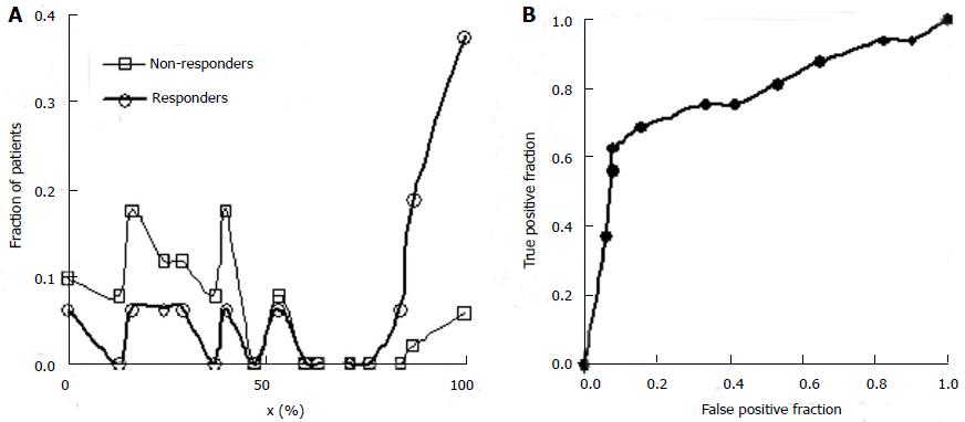
Columns 4 and 5 from the left in Table 3 give the fractions of non-responders and responders to the experimental treatment in each class. These values are equivalent to the probability density function defined over the set of classes. Figure 7A shows the separation of responders and non-responders to the experimental treatment along the x-domain. The fraction of patients with each x-value is shown on the vertical axis. Patients with x-scores less than 50% respond better to the control treatment. Patients with x-scores over 80 percent respond better to the experimental treatment. These results alone suggest that future studies of the experimental drug for lung cancer focus on patients with x-scores of 60 or better. Other patients are not likely to benefit, and if these are included in future trial statistics, a larger N will be required to reject the null hypothesis at substantially greater time and cost.
By integrating the functions plotted in Figure 7A or constructing a running sum of values in Columns 4 and 5 of Table 3 one can obtain the true positive fractions and false positive fractions using expression (8) for patients for whom x equals or exceeds a cutoff value indicated in each row. The values of ffp and ftp are shown in the next two columns. From these values the ROC curve for screening (ftp as a function of ffp) can be plotted, as shown in Figure 7B. The values of ftp and ffp are needed to model the size and cost of the future clinical trial using equations (4), (5), and (6).
The value of parameter, q, is best estimated as the proportion of responders for all x-values, or the total of column 3 in Table 3 divided by the total of columns 2 and 3, namely
Math 39
= 16/67 = 0.24.
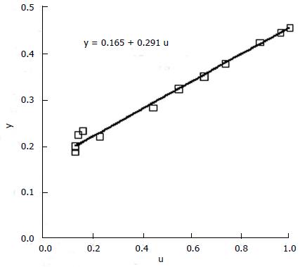
The values of parameters π3 and π4 are obtained by the regression analysis of expressions (9) through (12), using the control treatment data on the right of Table 3. The values in column 9, labeled pC|xc≥ x, are the conditional probabilities of response given that the cutoff value of x is at least as great as the x in any particular row. These values are important to explore, because patients that are likely to respond to the experimental drug may also tend to respond to the control treatment, being stronger by virtue of qualities not measured by x1 through x4. These probabilities π3 and π4 of response to control treatment can be estimated from regression analysis of derived variables u and y. The value of u in column 10 equals ffp/ftp , based upon the true positive and false positive fractions from experimental (not control) data. The value y in column 11 of Table 3 is the hybrid variable y = pC(u)(theta; + u). The slope of the regression line of a plot of y vs u is an estimate of π4, and the intercept divided by theta; = q(1 - q) is an estimate of π3.
Figure 8 shows the regression analysis on the rightmost two columns of Table 3. Both u and y are dimensionless. The intercept of the regression line is 0.165 and the slope is 0.291. Using expression (13), we have
Math 40
, and
Math 41
. The lumped control proportion of responders for all comers is 0.35. As expected, those classified as strong responders to the experimental treatment are also somewhat more likely to respond to the control treatment, an effect that should be accounted in modeling.
Parameters for the statistical model in this example are therefore q = 0.24, π1 = 1, π2= 0, π3 = 0.53, and π4 = 0.29.
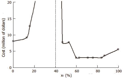
Figure 9 shows the corresponding cost function for model parameters q = 0.24, π1 = 1, π2.= 0, π3 = 0.53, and π4 = 0.29. Cost was computed using equations (4), (5), and (6) in succession. Cost coefficients are given in the figure legend.
This realistic example demonstrates that the choice of inclusion criteria can have a profound effect on the outcome of a clinical trial and that adjustment of inclusion criteria by quantitative means can produce protocols that achieve more with less. In Figure 9 the costs to the right of the dashed vertical asymptote correspond to a significant positive result with the experimental treatment better than control. Inclusion criteria of x > 60 points are likely to produce such outcomes. Costs to the left of the dashed vertical asymptote represent a significant negative result (experimental treatment worse than control). Inclusion criteria of x < 20 points would likely produce a significant negative outcome. The dashed vertical line represents selection criteria that would produce results entirely consistent with the null hypothesis.
A major challenge to medical innovation in the modern era is that when new improved drugs or other treatments are compared with reasonable, effective standard therapy, larger and larger trials are needed to detect incremental benefits at skyrocketing costs. If the effect of experimental treatment is borderline overall and strong in one subgroup, the overall conclusion is that the experimental treatment is not significantly different from control. The potential benefit in the favored subgroup is often not pursued, owing to limitations of time and cost.
This dilemma has led to the development of adaptive trial designs[9-14]. If investigators can determine early-on which types of patients are most likely to benefit from a novel treatment, then the trail can be re-targeted to favorable patients only. Alternatively, if a particular phenotype, such as the diabetic state, is found to have untoward complications compared to other types, then such patients can be excluded going forward, on a rational basis.
Here we show using a model-based approach how it is possible to minimize the time, cost, and probability of type II error of a clinical trial, by selection of optimal patient inclusion criteria. This approach provides a route to planning of a staged clinical trial for efficient use of resources in the confirmation stage of an adaptive trial design. It might even provide a way to resurrect good drugs or devices from failed trials by re-analysis of inclusion criteria used in the past.
The present model based approach can also be applied to data from one-armed preliminary trials of efficacy. Patients receiving the experimental treatment are characterized according to potential measures x1 through xk for tightened inclusion criteria. The distributions of values xi including all treated patients are tabulated and plotted for each metric, i. Continuous data such as age or fasting blood sugar concentration are dichotomized, based on inspection of the frequency distributions for responders vs non-responders to experimental treatment. Inherently dichotomous variables, such as male/female, or diabetic/non-diabetic are allowed also. Treated pilot patients are sorted into classes of putative responders and putative non-responders. Differences in proportions are used to construct a classifier (7), from which one can construct an ROC curve similar to Figure 3 using expression (8) that specifies possible pairs of ftp and ffp corresponding to different cutoffs for patient inclusion. These values, together with those of π3, π4 and q, estimated as described from pilot data and/or from the literature for standard (control) therapy, allow construction of the cost function (6) and identification of minimal cost inclusion criteria going forward.
The present work builds upon the rich literature describing adaptive clinical trial designs. An adaptive design allows the users to modify a trial during its progress based on interim results without affecting the validity and integrity of the trial. There are several subtypes of adaptive designs[15]. A group Sequential design allows for premature termination of a trial based on evidence of strong efficacy or futility at interim analyses. If a trial shows a positive result at an early stage, the trial is stopped, leading to an earlier launch of the new drug. If trail shows a negative result, early stopping avoids wasting resources. Sequential methods typically lead to savings in sample size, time, and cost when compared to the classical design with a fixed sample size[16].
Adaptive design with sample size re-estimation based upon interim results avoids inaccurate estimation of the effect size and its variability, which can lead to an underpowered or overpowered study. If a trial is underpowered, it will not be able to detect a clinically meaningful difference, and consequently could prevent a potentially effective drug from being delivered to patients. If a trial is overpowered, it could lead to unnecessary exposure of many patients to a potentially harmful compound when the drug, in fact, is not effective. Adaptive sample size re-estimation avoids these pitfalls and can reduce the expected sample size, and in turn the cost of the study, under a range of treatment effects. Protocols and procedures for re-specification of sample size are well described in the literature[4,17-21]. This type of adaptive design can arguably reduce time and cost, but does not specifically deal with optimizing inclusion/exclusion criteria.
Other forms of adaptation deal with allocation of patients to particular treatment groups. A drop-the-loser design is an adaptive design consisting of multiple stages. At each stage, interim analyses are performed and the losers (i.e., inferior treatment groups) are dropped. Note that this approach does not deal with patient selection but with treatment selection. Alternatively, a play-the-winner design increases allocation to successful treatments, based upon preliminary results. This form of adaptive design is most useful in multiple-arm or dose-ranging trials. They allow a shared control group, dropping of ineffective treatments before the end of the trial and stopping the trial early if sufficient evidence of a treatment being superior to control is found[22]. These now classical kinds of adaptive designs refine how many randomly selected patients are placed in known treatment groups. They do not refine patient selection criteria based upon biomarkers or traits that contain information about how individual patients are likely to respond to individual treatment.
Biomarker adaptive designs, currently being developed, allow adaptations according to biomarkers that indicate biologic or pharmacologic response to a therapeutic intervention. In one application biomarkers may serve as surrogate end points that predict outcomes such as long-term survival[23]. In another application, envisioned in the present study, biomarkers can be used to select the most appropriate target population. Recently, Jiang et al[24] proposed a statistically rigorous biomarker-adaptive threshold phase III design, in which a putative biomarker is used to identify patients who are sensitive to the new agent. The biomarker is measured on a continuous or graded scale, and a cut point established to define the sensitive subpopulation. Using a proportional hazards model that describes the relationship among outcome, treatment, and biomarker value for a two-treatment clinical trial, they found that when the proportion of sensitive patients as identified by the biomarker is low, the proposed design provided a substantial improvement in efficiency compared with the traditional trial design. Drs. Freidlin et al[9] proposed a new adaptive design for randomized clinical trials of targeted agents in settings where an assay or signature that identifies sensitive patients is not available at the outset of the study. They concluded that when the proportion of patients sensitive to the new drug is low, the adaptive design substantially reduces the chance of false rejection of effective new treatments. This prior work, as well as the present study, supports the idea that biomarkers can add substantial value to current medical practice by guiding patient-specific treatment selection in the conduct of clinical trials[25].
As such biomarker adaptive trial designs become implemented, more patients will receive a treatment that is effective for them. Fewer useful therapies for carefully selected patients will be lost to further development. The transition from bench to bedside will be faster, future patients awaiting better treatments will have less time to wait, and the high cost of conducting clinical trials will be minimized.
Let the linear classifier
Math 42
for dichotomous predictive variables
Math 43
and for xi independent or poorly correlated, based upon pilot data. Treat the coefficients, ai, as variables to be optimized for best discrimination of non-responders, NR, from responders, R. The mean values from pilot data for these subgroups are
Math 44
and
Math 45
, and the difference in means between responders and non-responders for the classifier is
Math 46
For dichotomous variables the mean value
Math 47
is the equal to the proportion, piR, of responders for whom xi = 1, and mean value
Math 48
is the equal to the proportion, piNR, of non-responders for whom xi = 1. Then
Math 49
for constants, bi, derived from pilot data.
Let V(X) = the variance of random variable, X, and let us choose the ai so that
Math 50
is maximized as a measure of the separation of classes NR and R in the x-domain. Here the variance estimate from the given pilot data representing nNR non-responders and nR responders to experimental therapy (with independent xi) is
Math 51
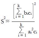
for constants, ci, derived from pilot data. Hence, using the estimate for the variance in the denominator,
Math 52
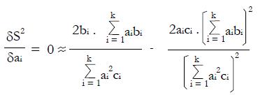
To maximize (or minimize) S2 in the a1, a2, ¡. ak domain, we can solve the set of normal equations δS2/δa1 = 0, δS2/δa2 = 0,... δS2/δa1 = 0 obtained by setting the partial derivatives equal to zero, where for any particular dichotomous variable, i,
Math 53
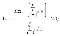
or
Math 54
for i = 1, 2, ¡ k,
which gives a set of k equations with k unknown variables, ai, and 2k known variables, bi and ci, derived from the pilot data.
Two solutions are evident from simple inspection of the forgoing normal equations. Trivially, if bi = 0 for all i, that is if piR = piNR, then we have a minimum with
Math 55
. However, if ai = bi = piR - piNR , and if ci ≈ c, a constant (as is reasonable from inspection of the expression for the variance of proportions not too close to zero or one), we have an approximate solution to the normal equations for a maximum S2, given the bi≠ 0 and ci≠ 0 from the training data. Thus we can expect roughly maximal separation of populations NR and R in the x domain if
ai = bi = piR - piNR,
the differences in proportions of responders vs non-responders having dichotomous variable scores xi = 1.
Although we assume that the xi are poorly correlated, it can be shown numerically that this choice of the ai is insensitive to small inter-correlations between predictors, x. If two predictors are strongly correlated, they can be combined into a single predictor, for example, high serum creatinine and high blood urea nitrogen can be lumped as “renal insufficiency”, reducing the number of dimensions, k. Lumping highly correlated parameters in this way can improve separation of the classes NR and R and can avoid undesired over-weighting of the property measured by both correlated variables.
Clinical trials are too costly and take too long to complete. High costs of clinical trials add significantly to the ultimate costs of new medicines and medical devices. Delay in completion of a trial due to inefficient trial design can postpone, sometimes indefinitely, the transfer of promising new therapies from bench to bedside.
The treatment of cancer, in particular, is moving towards the use of more specific therapies that are targeted to each tumor type. To facilitate this shift, tests are being developed to link specific genetic variations to specific drug effects using biomarkers that help predict how a given individual will respond to a drug.
This paper demonstrates how one can use biomarkers and other patient characteristics from a one-armed Phase II study or early-stage pilot data from an adaptive trail design to create a suitable classifier for discriminating responders from non-responders to a test drug or treatment.
Sample calculations using reconstructed raw data for a study of a novel drug treatment for lung cancer demonstrate that the choice of inclusion criteria can have a profound effect on the outcome of a clinical trial and that adjustment of inclusion criteria by quantitative means can produce protocols that achieve more with less. This example shows, using a model-based approach, how to minimize the time and cost of a clinical trial by selection of optimal patient inclusion criteria. Clear cost minimums exist for realistic scenarios with potential cost savings in millions of dollars. As the response rate for controls approaches 50%, the proper choice of inclusion criteria can mean the difference between a successful trial and a failed trial, no matter what the cost.
Adaptive trial design: a clinical trial design that allows modification of aspects of the trial as it continues, based upon accumulating data in a statistically and intellectually valid way. Type II statistical error: failure to reject the null hypothesis when it is false, that is, a false negative interpretation of a research study.
The topic is novel and one that is much welcomed in this space. The thinking is in the right direction.
P- Reviewer: Iyngkaran P S- Editor: Gou SX L- Editor: A E- Editor: Wu HL
| 1. | Anderson JE, Hansen LL, Mooren FC, Post M, Hug H, Zuse A, Los M. Methods and biomarkers for the diagnosis and prognosis of cancer and other diseases: towards personalized medicine. Drug Resist Updat. 2006;9:198-210. [RCA] [PubMed] [DOI] [Full Text] [Cited by in Crossref: 50] [Cited by in RCA: 52] [Article Influence: 2.7] [Reference Citation Analysis (0)] |
| 2. | Ross JS, Slodkowska EA, Symmans WF, Pusztai L, Ravdin PM, Hortobagyi GN. The HER-2 receptor and breast cancer: ten years of targeted anti-HER-2 therapy and personalized medicine. Oncologist. 2009;14:320-368. [RCA] [PubMed] [DOI] [Full Text] [Cited by in Crossref: 850] [Cited by in RCA: 846] [Article Influence: 52.9] [Reference Citation Analysis (0)] |
| 3. | van’t Veer LJ, Bernards R. Enabling personalized cancer medicine through analysis of gene-expression patterns. Nature. 2008;452:564-570. [RCA] [PubMed] [DOI] [Full Text] [Cited by in Crossref: 398] [Cited by in RCA: 364] [Article Influence: 21.4] [Reference Citation Analysis (0)] |
| 4. | Yao Q, Wei LJ. Play the winner for phase II/III clinical trials. Stat Med. 1996;15:2413-223; discussion 2413-223;. [PubMed] |
| 5. | Bauer P, Köhne K. Evaluation of experiments with adaptive interim analyses. Biometrics. 1994;50:1029-1041. [RCA] [PubMed] [DOI] [Full Text] [Cited by in Crossref: 627] [Cited by in RCA: 553] [Article Influence: 18.4] [Reference Citation Analysis (0)] |
| 6. | Babbs CF. Simplified meta-analysis of clinical trials in resuscitation. Resuscitation. 2003;57:245-255. [RCA] [PubMed] [DOI] [Full Text] [Cited by in RCA: 1] [Reference Citation Analysis (0)] |
| 7. | Cooper BE. Statistics for Experimentalists. 1st ed. Oxford: Permagon Press Ltd 1969; . |
| 8. | Shaw AT, Yeap BY, Mino-Kenudson M, Digumarthy SR, Costa DB, Heist RS, Solomon B, Stubbs H, Admane S, McDermott U. Clinical features and outcome of patients with non-small-cell lung cancer who harbor EML4-ALK. J Clin Oncol. 2009;27:4247-4253. [RCA] [PubMed] [DOI] [Full Text] [Cited by in Crossref: 1345] [Cited by in RCA: 1511] [Article Influence: 94.4] [Reference Citation Analysis (0)] |
| 9. | Freidlin B, Simon R. Adaptive signature design: an adaptive clinical trial design for generating and prospectively testing a gene expression signature for sensitive patients. Clin Cancer Res. 2005;11:7872-7878. [RCA] [PubMed] [DOI] [Full Text] [Cited by in Crossref: 275] [Cited by in RCA: 234] [Article Influence: 12.3] [Reference Citation Analysis (0)] |
| 10. | Coffey CS, Kairalla JA. Adaptive clinical trials: progress and challenges. Drugs R D. 2008;9:229-242. [RCA] [PubMed] [DOI] [Full Text] [Cited by in Crossref: 55] [Cited by in RCA: 48] [Article Influence: 2.8] [Reference Citation Analysis (0)] |
| 11. | Howard G. Nonconventional clinical trial designs: approaches to provide more precise estimates of treatment effects with a smaller sample size, but at a cost. Stroke. 2007;38:804-808. [RCA] [PubMed] [DOI] [Full Text] [Cited by in Crossref: 12] [Cited by in RCA: 9] [Article Influence: 0.5] [Reference Citation Analysis (0)] |
| 12. | Schäfer H. Adaptive designs from the viewpoint of an academic biostatistician. Biom J. 2006;48:586-590; discussion 613-622. [RCA] [PubMed] [DOI] [Full Text] [Cited by in Crossref: 3] [Cited by in RCA: 3] [Article Influence: 0.2] [Reference Citation Analysis (0)] |
| 13. | Hung HM, O’Neill RT, Wang SJ, Lawrence J. A regulatory view on adaptive/flexible clinical trial design. Biom J. 2006;48:565-573. [RCA] [PubMed] [DOI] [Full Text] [Cited by in Crossref: 60] [Cited by in RCA: 51] [Article Influence: 2.7] [Reference Citation Analysis (0)] |
| 14. | Müller HH, Schäfer H. Adaptive group sequential designs for clinical trials: combining the advantages of adaptive and of classical group sequential approaches. Biometrics. 2001;57:886-891. [RCA] [PubMed] [DOI] [Full Text] [Cited by in Crossref: 278] [Cited by in RCA: 250] [Article Influence: 10.4] [Reference Citation Analysis (0)] |
| 15. | Chang M. Classical and Adaptive Clinical Trial Designs Using ExpDesign Studio. Bangkok: John Wiley & Sons 2008; 260. |
| 16. | Vandemeulebroecke M. Group sequential and adaptive designs - a review of basic concepts and points of discussion. Biom J. 2008;50:541-557. [RCA] [PubMed] [DOI] [Full Text] [Cited by in Crossref: 28] [Cited by in RCA: 28] [Article Influence: 1.6] [Reference Citation Analysis (0)] |
| 17. | Ohrn F, Jennison C. Optimal group-sequential designs for simultaneous testing of superiority and non-inferiority. Stat Med. 2010;29:743-759. [RCA] [PubMed] [DOI] [Full Text] [Cited by in Crossref: 13] [Cited by in RCA: 13] [Article Influence: 0.9] [Reference Citation Analysis (0)] |
| 18. | Cui L, Hung HM, Wang SJ. Modification of sample size in group sequential clinical trials. Biometrics. 1999;55:853-857. [RCA] [PubMed] [DOI] [Full Text] [Cited by in Crossref: 360] [Cited by in RCA: 337] [Article Influence: 13.0] [Reference Citation Analysis (0)] |
| 19. | Jennison C, Turnbull BW. Mid-course sample size modification in clinical trials based on the observed treatment effect. Stat Med. 2003;22:971-993. [RCA] [PubMed] [DOI] [Full Text] [Cited by in Crossref: 148] [Cited by in RCA: 114] [Article Influence: 5.2] [Reference Citation Analysis (0)] |
| 20. | Li G, Shih WJ, Xie T, Lu J. A sample size adjustment procedure for clinical trials based on conditional power. Biostatistics. 2002;3:277-287. [RCA] [PubMed] [DOI] [Full Text] [Cited by in Crossref: 78] [Cited by in RCA: 79] [Article Influence: 3.4] [Reference Citation Analysis (0)] |
| 21. | Schäfer H, Timmesfeld N, Müller HH. An overview of statistical approaches for adaptive designs and design modifications. Biom J. 2006;48:507-520. [RCA] [PubMed] [DOI] [Full Text] [Cited by in Crossref: 20] [Cited by in RCA: 20] [Article Influence: 1.1] [Reference Citation Analysis (0)] |
| 22. | Wason JM, Jaki T. Optimal design of multi-arm multi-stage trials. Stat Med. 2012;31:4269-4279. [RCA] [PubMed] [DOI] [Full Text] [Cited by in Crossref: 80] [Cited by in RCA: 80] [Article Influence: 6.2] [Reference Citation Analysis (0)] |
| 23. | Weir CJ, Walley RJ. Statistical evaluation of biomarkers as surrogate endpoints: a literature review. Stat Med. 2006;25:183-203. [PubMed] |
| 24. | Jiang W, Freidlin B, Simon R. Biomarker-adaptive threshold design: a procedure for evaluating treatment with possible biomarker-defined subset effect. J Natl Cancer Inst. 2007;99:1036-1043. [RCA] [PubMed] [DOI] [Full Text] [Cited by in Crossref: 192] [Cited by in RCA: 158] [Article Influence: 8.8] [Reference Citation Analysis (0)] |
| 25. | Mandrekar SJ, Sargent DJ. Clinical trial designs for predictive biomarker validation: theoretical considerations and practical challenges. J Clin Oncol. 2009;27:4027-4034. [RCA] [PubMed] [DOI] [Full Text] [Cited by in Crossref: 314] [Cited by in RCA: 272] [Article Influence: 17.0] [Reference Citation Analysis (0)] |


