State of machine and deep learning in histopathological applications in digestive diseases

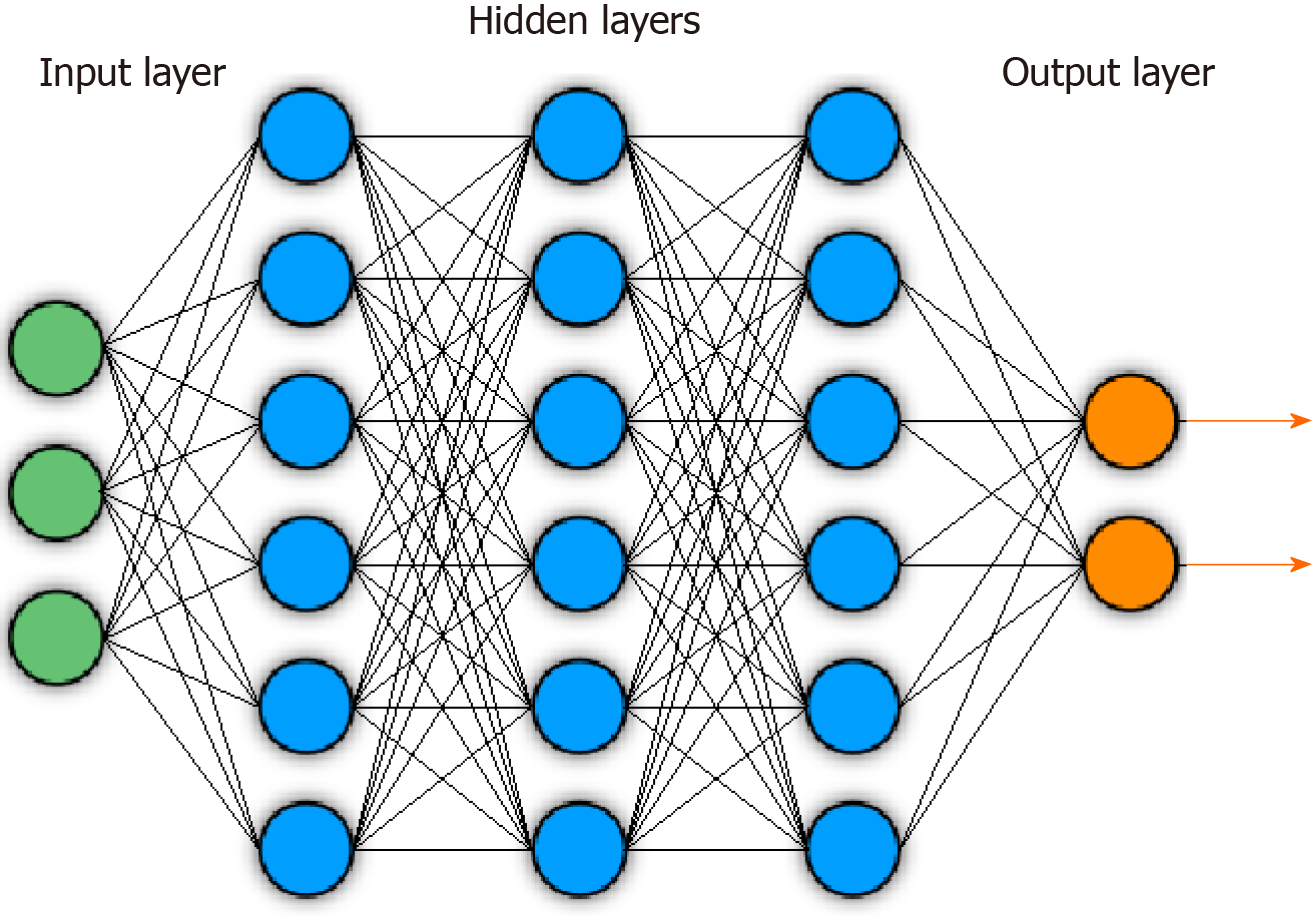
Figure 1 Example of general deep neural network architecture. Circles indicate nodes. Lines indicate feeding of layer node outputs into next layer nodes.

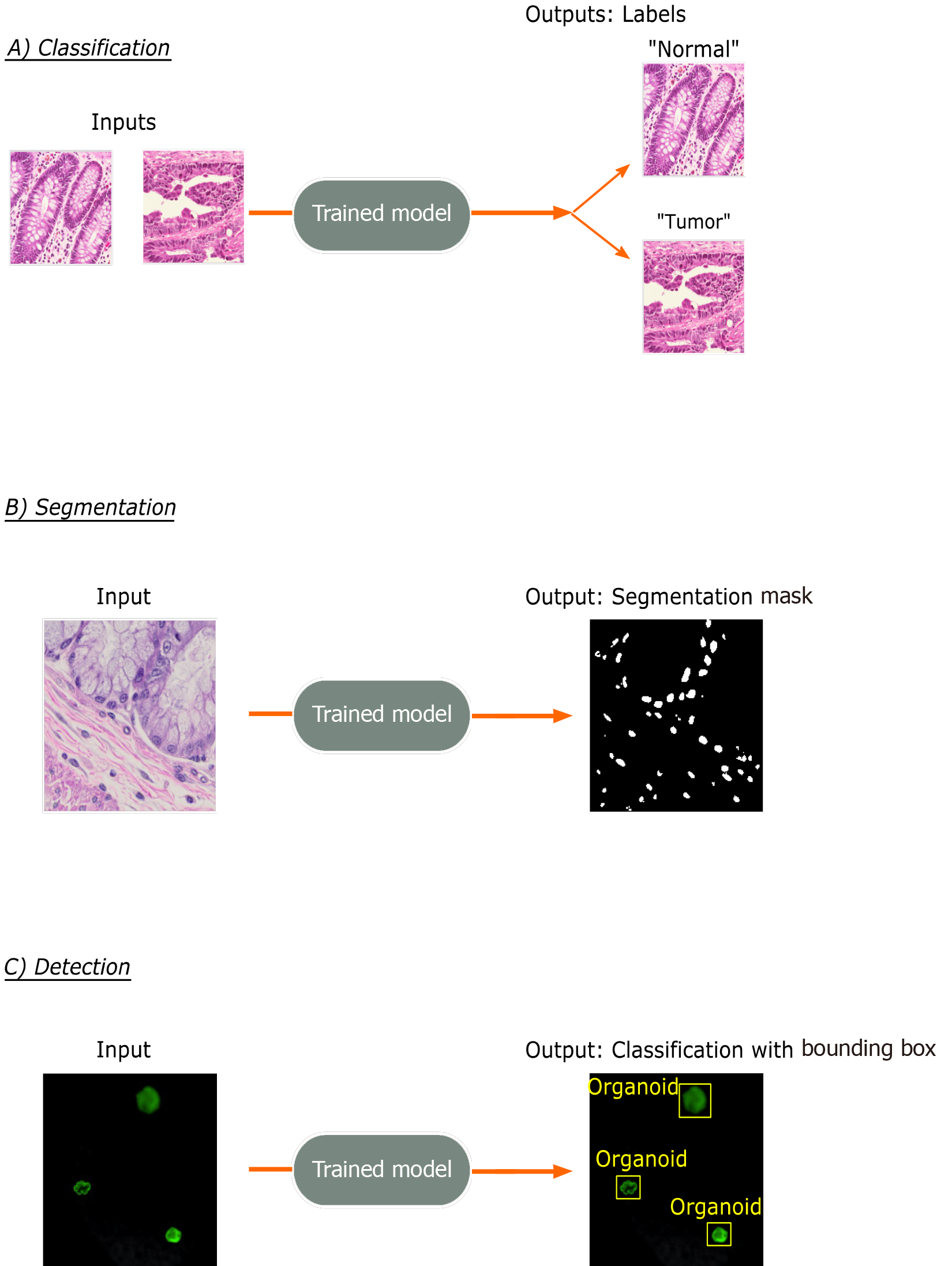
Figure 2 Common trainable tasks by deep learning. A: Classification involves designation of a class label to an image input. Image patches for the figure were taken from colorectal cancer and normal adjacent intestinal samples obtained via an IRB-approved protocol; B: Segmentation tasks output a mask with pixel-level color designation of classes. Here, white indicates nuclei and black represents non-nuclear areas; C: Detection tasks generate bounding boxes with object classifications. Immunofluorescence images of mouse-derived organoids with manually inserted classifications and bounding boxes in yellow are included for illustrative purposes.

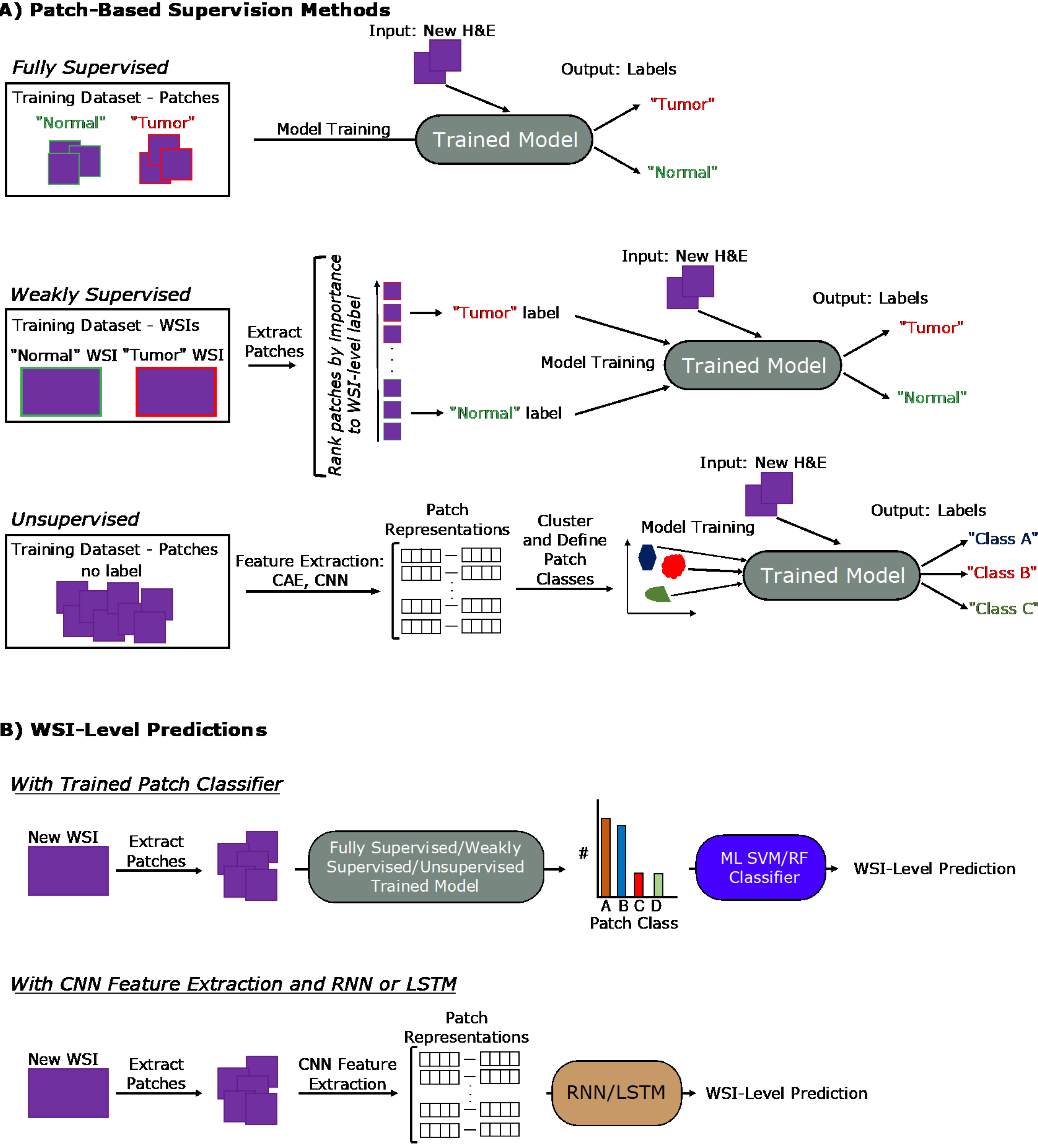
Figure 3 General deep learning training and prediction approaches. A: Examples pipelines for fully supervised, weakly supervised, and unsupervised learning methods for training patch classifiers are shown; B: Two pipelines translating patch-level information into whole-slide image-level predictions are shown. The top approach utilizes a patch classifier trained by one of the approaches in (A). The bottom approach uses a convolutional neural network feature extractor to generate patch representations that are fed into a long short-term memory or recurrent neural network. H&E: Hematoxylin and eosin; WSI: Whole-slide image; CNN: Convolutional neural network; RNN: Recurrent neural network; LSTM: Long short-term memory; CAE: Convolutional autoencoder.

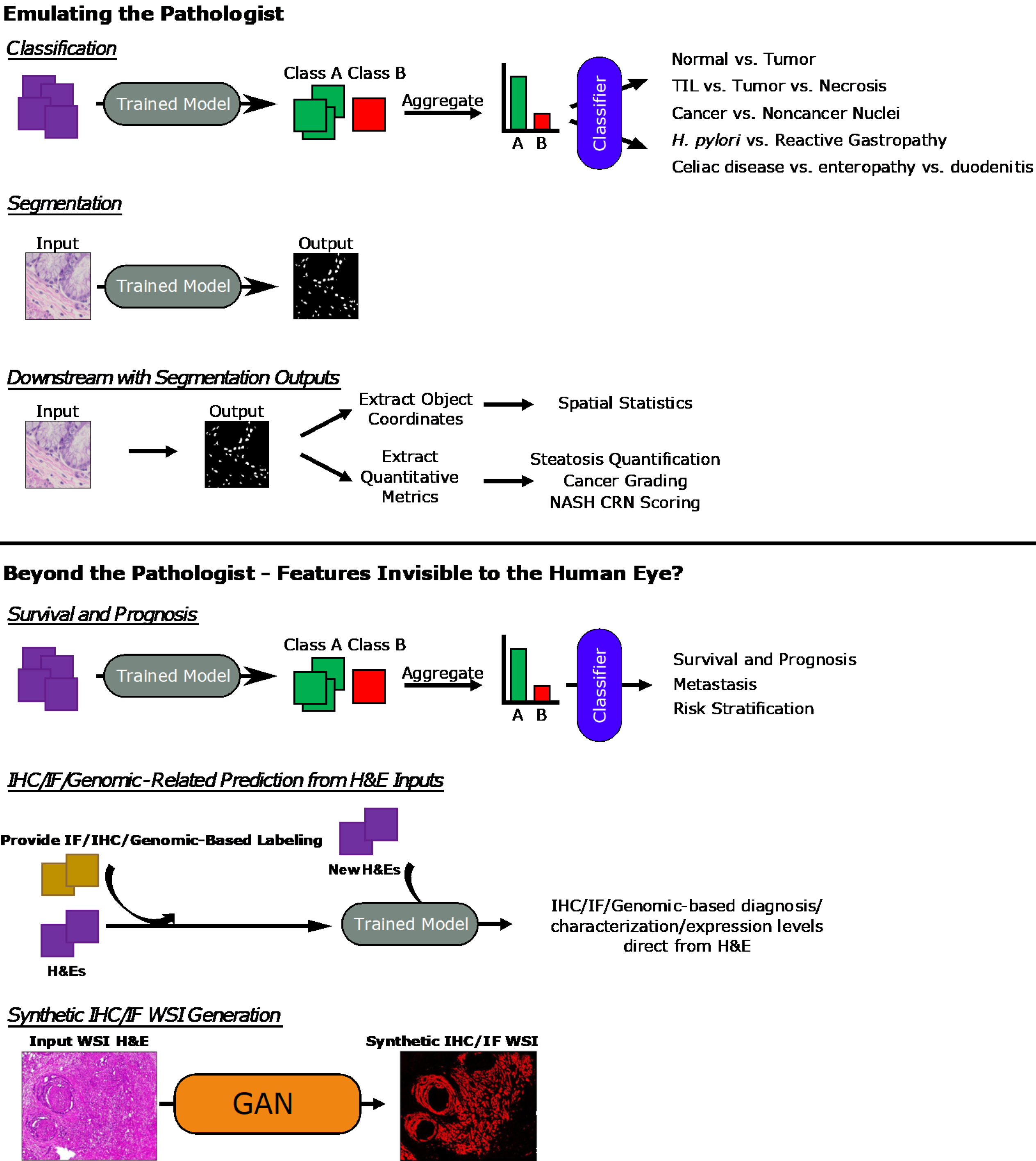
Figure 4 General overview of approaches. Overview of general machine learning - and deep learning-based approaches covered in the sections of this review are presented here. Whole-slide image (WSI) hematoxylin and eosin and Synthetic immunofluorescence (IF) WSI images in the Synthetic immunohistochemistry/IF Generation pipeline. Citation: Burlingame EA, McDonnell M, Schau GF, Thibault G, Lanciault C, Morgan T, Johnson BE, Corless C, Gray JW, Chang YH. SHIFT: speedy histological-to-immunofluorescent translation of a tumor signature enabled by deep learning. Sci Rep 2020; 10: 17507. Copyright© The Authors 2020. Published by Springer Nature. TIL: Tumor-infiltrating lymphocyte; H. pylori: Helicobacter pylori; NASH CRN: Nonalcoholic Steatohepatitis Clinical Research Network; IHC: Immunohistochemistry; IF: Immunofluorescence; H&E: Hematoxylin and eosin; WSI: Whole-slide image; GAN: General adversarial network.

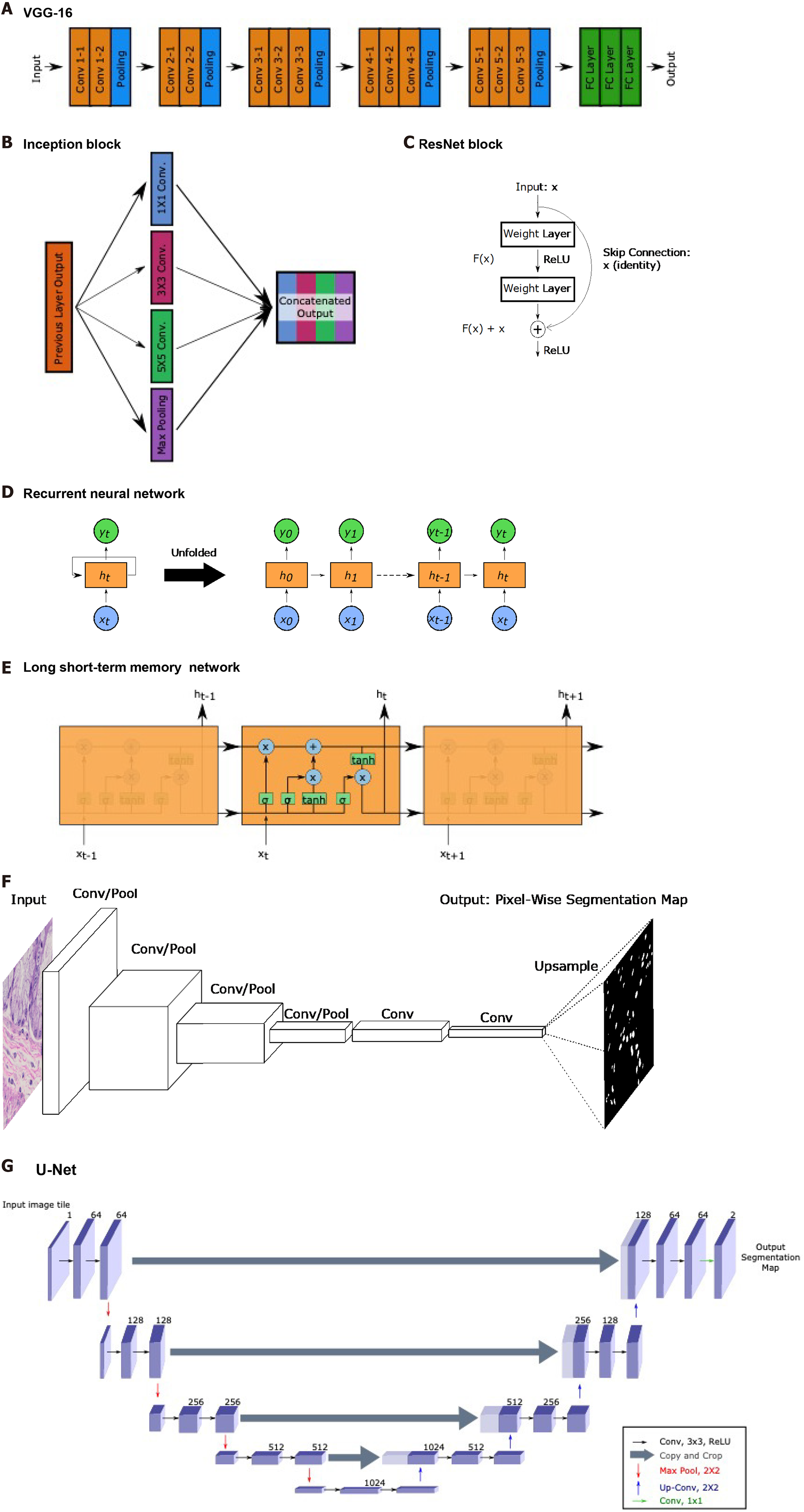
Figure 5 Common landmark network architectures. Overviews of landmark network architectures utilized in this paper are presented. A: The visual geometry group network incorporates sequential convolutional and pooling layers into fully connected layers for classification; B: The inception block utilized in the inception networks incorporates convolutions with multiple filter sizes and max pooling onto inputs entering the same layer and concatenates to generate an output; C: The residual block used in ResNet networks incorporates a skip connection; D: Recurrent neural networks (RNNs) have repeating, sequential blocks that take previous block outputs as input. Predictions at each block are dependent on earlier block predictions; E: Long short-term memory network that also has a sequential format similar to RNN. The horizontal arrow at the top of the cell represents the memory component of these networks; F: Fully convolutional networks perform a series of convolution and pooling operations but have no fully-connected layer at the end. Instead, convolutional layers are added and deconvolution operations are performed to upsample and generate a segmentation map output of same dimensions as the input. Nuclear segmentation images are included for illustration purposes; G: U-Net exhibits a U-shape from the contraction path that does convolutions and pooling and from the decoder path that performs deconvolutions to upsample dimensions. Horizontal arrows show concatenation of feature maps from convolutional layers to corresponding deconvolution outputs. VGG: Visual geometry group.

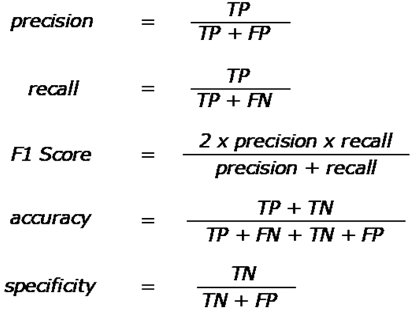
Figure 6 Quantitative performance metric equations. Quantitative metrics are based off of true positive, true negative, false positive, and false negative counts from results. Equations for precision, recall, F1 score, accuracy, and specificity. Precision is also known as the true positive rate, and recall is also known as sensitivity. TP: True positive; TN: True negative; FP: False positive; FN: False negative.